[khebab]

To my current knowledge there´s none.
(just sharing a little 2+2=4 here:)
Just assume that separate areas of knowledge (financial, physical and energy related, in this case) connect at some point, and keep researching.

Thanks for the hints, I know that P/Q vs Q have been used aslo for population study. By the way, do you have a link for the first image you posted before.

Extra Hint:
The simulation using the sum of a hubbert curve and a constant amplitude cosine wave is useful to reach the conclusion that the linearization process narrows along time, but, when comparing with real models, it´s possible to conclude that this simulation doesn´t narrow as fast as the real ones.
i suggest a simulation using a DAMPED cosine wave, where it´s possible to adjust the damping factor to fit the curve better for comparison with true and real measurements (like Norway´s) without "human adjusted" factors.
more on this later....

Ok but it seems that the damping occurs naturally in P/Q because of the division by an increasing Q. I'm not sure I fully understand your comment.

[khebab]

but one could object than you take as guaranted that production is generally hubbert-shaped, with some random variations around the base hubbert curve.

Yes it is the main assumption here.

There are countries where production is not Hubbert-shaped at all, for one of the following reasons :
# Production quotas (opec countries)
# disruption by war, embargo (Iraq), political collapse (FSU)
# several distinct production zones with large time lag, then production can be modelled as the sum of two or more hubbert cycles.
# production is constrainbed by pipeline capacity (Chad, Ecuador...).

Agreed, production modeling is really difficult for some countries especially when production is immature and the YTF is still important (ex: Nigeria) with possibly multiple Hubbert cycles involved.

Now, according to your results, if the production is "free" (no constraint => hubbert shape), we can have a reasonnably good estimation of URR even with only the 20% first percents of it gone. Then perharps we could get some rough estimation of Middle East's ultimate using figures up to 1980, before the quota were established ?

hmm... the confidence level at 20% of Qinf is rather low (~20%).

Where could I find historical figures excludin refinery gain? It would be even better to have a split into crude, NGL's, and non-conventionnal production.

Finding good and reliable data is a big issue, some private database (ex: IHS) have probably this level of details.

[rrb]

Actually that brings up a very good point. The peak region is the only meaty part of the fit. Any curve that has a parabolic fit around the peak will give a good Hubbert Linearization. And since every symmetric peak is approximated by an upside-down parabola (i.e. quadratic) due to Taylor-series, that means that just about any peaked curve will work.

Does this suggest that the linearization will not be very
good at the tail end in case the whole curve is not quadratic?
In that case, the estimate of the URR based on the linearization
may be quite a bit off. It also explains the poor approximation
at the start of the curve.

[WebHubbleTelescope]

Actually that brings up a very good point. The peak region is the only meaty part of the fit. Any curve that has a parabolic fit around the peak will give a good Hubbert Linearization. And since every symmetric peak is approximated by an upside-down parabola (i.e. quadratic) due to Taylor-series, that means that just about any peaked curve will work.

Does this suggest that the linearization will not be very
good at the tail end in case the whole curve is not quadratic?
In that case, the estimate of the URR based on the linearization
may be quite a bit off. It also explains the poor approximation
at the start of the curve.

Actually, it works perfectly over the whole range only for the logistic curve. That is the interesting property of the logistic curve. How this came about is through a sequence of steps:
1. Somebody notices the production curve kind of fits a logistics curve
2. Somebody notices the logistic curve linearizes nicely when plotted a certain way.
3. Lots of people start plotting production curves this way.
4. Everyone nods their head in agreement, ignoring the fact that it actually doesn't fit over the entire range anyways

This next step hasn't happened yet.
5. Other models will work just as well over a certain range, thus making the logistic curve just another interesting empirical relationship.

[WebHubbleTelescope]

BTW, thanks Khebab for starting this thread.

What you are doing -- shaking the tree and seeing what falls off or gets wobbly -- is exactly the right approach to finding the weaknesses.

[bantri]

By the way, do you have a link for the first image you posted before.

It´s gone, it´s an indirect link that i´ve spotted it when i was searching for black scholes keywords in the images section of google.

the most similar one is being displayed in wikipedia, but the exponential funnel is different (less damped, and ramping up)

http://de.wikipedia.org/wiki/Bild:Black ... ta_ttm.png
http://de.wikipedia.org/wiki/Black-Scholes-Modell

Ok but it seems that the damping occurs naturally in P/Q because of the division by an increasing Q. I'm not sure I fully understand your comment.

indeed it happens mathematically, but try consider also a physical point of view, exponential damping also happens in decaying energy systems.

if you put a resistor R in an LC circuit, and start to dissipate the initial energy given inside the system to the outside, in the form of heat, the oscilations may be random but they are contained inside a narrowing exponential funnel.

[khebab]

Motivation:

This thread is a continuation of How Reliable is the Hubbert Linearization Method?. The main motivation here is again to gain some insight in the robusteness, the limitations of the curve fitting aproach. One main issue is the lack of confidence intervals on crucial parameters (Ultimate Recoverable Ressource, growth rate and peak date).

What is bootstrapping? it's a way to repeat an experiment. With the Bootstrap, a new set of experiment is not needed, the original data is reused. Specifically, the original observations are randomly reassigned and the estimate is recomputed. These assignments and recomputations are done a large number of times and considered as repeated assignements.

Why is the bootstrap attractive? It can answer many questions with very little in the way of modelling, assumptions and can be applied easily.

In general, the bootstrap is a methodology for answering the following question: How accurate is a parameter estimator?. Bootstrapping is a fairly new method in statistics and has been proposed by Efron in 1979. The R software (open source ) has a bootstrap library called 'boot' that implements almost all the standard techniques. I won't go into the details of the Bootstrap theory, a lot of details about the techniques and the R language implementation used in this post can be found in the following document:

John Fox. Bootstrapping Regression Models, Appendix to an R and S-plus Companion to Applied Regression

Application:

I restate the Hubbert linearization equation:

Code: Select all

P(t)/Q(t)= K(1 - Q(t)/URR)

where Q(t) is the cumulative production at time t, K is the growth rate and URR=Q(t=+inf) (for a good discussion on this approach: Another Way of Looking at CERA).

The BP production data are used for the world production.

For each starting year Y we randomly generate 2,000 new samples (called bootstrap replicates) taken in the time range [Y:2004] on which a robust least-square fitting is perfomed (function rlm).

[align=center]
large version
(a) URR

large version
(b) K
Histograms and normal quantile-comparison plots for the bootstrap replications of the URR (a) and K (b). The broken vertical line in each histogram shows the original value for the model fit to the original sample.[/align]

The confidence intervals are derived from the bootstrap replicates using the so-called bias-corrected accelerated method (BCa). The R script is given in the post below and has produced the following numerical results.

Code: Select all

   Y    URR(50%)U URR(50%)L  K(50%)L  K(50%)U    URR(90%)L URR(90%)U  K(90%)L   K(90%)U   URR(95%)L URR(95%)U  K(95%)L     K(95%)U
1  1940 1589.852 1666.108 0.06553184 0.06803704 -1047.8955 1722.340 0.06229963 0.07005338 -2115.754 1738.640 0.05931496 0.07057659
2  1945 1534.121 1604.606 0.06716867 0.06970711  -909.1412 1655.086 0.06448430 0.07143187 -1694.621 1674.993 0.06099418 0.07215952
3  1950 1474.262 1535.714 0.06936133 0.07203309  1415.9148 1580.065 0.06720602 0.07404873  1371.762 1593.248 0.06624411 0.07463725
4  1955 1411.245 1479.824 0.07170182 0.07469338  1358.8073 1529.928 0.06909329 0.07690102  1332.695 1570.994 0.06755400 0.07777587
5  1960 1344.488 1429.857 0.07396238 0.07755941  1288.4431 1999.462 0.05258170 0.08004962  1269.352 2069.939 0.05197241 0.08069580
6  1965 1251.694 1362.724 0.07767415 0.08219249  1127.0189 2032.670 0.05220087 0.08584747  1048.126 2077.450 0.05171007 0.08775371
7  1970 1867.918 2100.396 0.05173704 0.05643942  1248.4862 2169.640 0.05066231 0.08498707  1150.549 2186.294 0.05038610 0.08823982
8  1975 2016.554 2132.814 0.05118828 0.05302772  1827.8085 2199.954 0.05023261 0.05699570  1443.484 2219.633 0.04985585 0.07501213
9  1980 2048.701 2138.568 0.05113436 0.05246769  1920.1593 2201.945 0.05022459 0.05480756  1837.808 2223.453 0.04995022 0.05584261
10 1985 2124.600 2202.525 0.05005941 0.05111410  2015.7552 2273.314 0.04894792 0.05221503  1840.982 2353.670 0.04681022 0.05449696

from which we derive the following figures:
[align=center]

[/align]
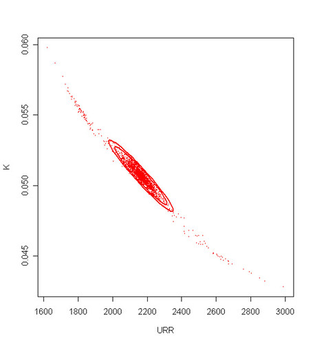
We can also look at the correlation between the bootstrap replicates of the K and URR coeffcients:
[align=center]
Scatterplot of the bootstrap replications of the URR and K coefficients for the BP data. The concentrations ellipse are drawn at 50, 90, and 99% level using a robust estimate of the covariance matrix of the coefficients[/align]
Discussion:

1- The 95% confidence intervals for the URR and K using data from 1980 to 2004 is [1838.0 2223.0] Gb and [5.0 5.6]% respectively.
2- Not surprisingly, the confidence intervals are strongly affected by the 70's hump in production. The 1965-1970 period constitutes a transition or shock period between two production regimes.
3- Estimates from data starting around 1970 are fairly stable
4- the parameter K is negatively correlated with the URR (higher K values will give lower URR)
5- Many variations can be made, for instance in the way the robust least-square is applied

[khebab]

Enjoy!

Code: Select all

####################################################################
##
##  Script that illustrate bootstrapping techniques applied
##  to the Hubbert linearization of the total world production.
##
##  see the thread http://www.peakoil.com/fortopic16349.html for more details
## 
##  Author: Khebab (January, 2006)
##  version 1.0
##
####################################################################

rm(list=ls(all=TRUE))   # clean up
##
##  Load matlab emulator package and gremisc (to install)
##  in the menu bar: packages/install pacakage(s)
##
library(matlab)
library(gregmisc)
library(boot)
library(MASS)
library(car)

####################################################################
##
##              Main
##
####################################################################

#
#   World oil production since 1901 up to 2005 (from BP) in Gb (all liquids)
#
temp <- scan()
2.0000000e-001  1.6740000e-001  1.8180000e-001  1.9490000e-001  2.1800000e-001  2.1510000e-001 
2.1330000e-001  2.6420000e-001  2.8560000e-001  2.9870000e-001  3.2780000e-001  3.4440000e-001 
3.5240000e-001  3.8530000e-001  4.0750000e-001  4.3200000e-001  4.5750000e-001  5.0290000e-001 
5.0350000e-001  5.5590000e-001  6.8890000e-001  7.6600000e-001  8.5890000e-001  1.0157000e+000 
1.0143000e+000  1.0679000e+000  1.0968000e+000  1.2630000e+000  1.3250000e+000  1.4860000e+000 
1.4100000e+000  1.3730000e+000  1.3100000e+000  1.4420000e+000  1.5220000e+000  1.6540000e+000 
1.7920000e+000  2.0390000e+000  1.9880000e+000  2.0860000e+000  2.1500000e+000  2.2210000e+000 
2.0930000e+000  2.2570000e+000  2.5930000e+000  2.5950000e+000  2.7450000e+000  3.0220000e+000 
3.4330000e+000  3.4040000e+000  3.8030000e+000  4.2830000e+000  4.5190000e+000  4.7980000e+000 
5.0180000e+000  5.6260000e+000  6.1250000e+000  6.4390000e+000  6.6080000e+000  7.1340000e+000 
7.6613500e+000  8.1942500e+000  8.8877500e+000  9.5374500e+000  1.0285700e+001  1.1070450e+001 
1.2620000e+001  1.3550000e+001  1.4760000e+001  1.5930000e+001  1.7540000e+001  1.8560000e+001 
1.9590000e+001  2.1340000e+001  2.1400000e+001  2.0380000e+001  2.2050000e+001  2.2890000e+001 
2.3120000e+001  2.4110000e+001  2.2980000e+001  2.1730000e+001  2.0910000e+001  2.0660000e+001 
2.1050000e+001  2.0980000e+001  2.2070000e+001  2.2190000e+001  2.3050000e+001  2.3380000e+001 
2.3900000e+001  2.3830000e+001  2.4010000e+001  2.4110000e+001  2.4500000e+001  2.4860000e+001 
2.5510000e+001  2.6340000e+001  2.6860000e+001  2.6400000e+001  2.7360000e+001  2.7310000e+001 
2.7170000e+001  2.8120000e+001 

vWorldProduction <- matrix(temp, ncol=1 , byrow= F)


mProductionData <- cbind(cbind(c(1901:2004), vWorldProduction), cumsum(vWorldProduction));
mProductionData <- cbind(mProductionData, mProductionData[,2]/mProductionData[,3])

colnames(mProductionData , do.NULL = FALSE)
colnames(mProductionData )<- c("Year","Prod","CumProd","PQ")
frProductionData <- data.frame(year= mProductionData[, 1],  prod = mProductionData[,2], cumprod= mProductionData[,3], pq= mProductionData[,4])

head(frProductionData)
#
#   Function that apply the Hubbert linearization technique
#
boot.RLS.twoparam <- function(data, indices, maxit=20) {
   data <- data[indices,]
   mod <- rlm(pq ~ cumprod, data=data, maxit=maxit, method= "MM")
   v <- coefficients(mod)
   c(-v[1]/v[2], v[1])
}

matplot(x= frProductionData$cumprod, y= frProductionData$pq, pch = 1:4, type = "l", add= F, ylab= "P/q", xlab= "Q")
years <- c(1940,1945,1950,1955,1960,1965,1970,1975,1980,1985)
#years <- c(1940:1985)
Results.confidenceInterval <- data.frame(year= NA,
             URRMin1= NA, URRMax1= NA, KMin1= NA, KMax1= NA,
      URRMin2= NA, URRMax2= NA, KMin2= NA, KMax2= NA,
      URRMin3= NA, URRMax3= NA, KMin3= NA, KMax3= NA)
m <- 1
#
#   The bootstrapping technique is applied for different year intervals
#   from startingYear to 2004.
#
for(startingYear in years ) {
   
   idx <- find(frProductionData$year == startingYear)
   idx2 <- c(idx[1]:104)
   frSubProductionData <- data.frame(year= mProductionData[idx2 , 1],  prod = mProductionData[idx2 ,2],
             cumprod= mProductionData[idx2 ,3], pq= mProductionData[idx2 ,4]);
   # bootstrapping application
   Results.boot <- boot(frSubProductionData , boot.RLS.twoparam , 2000, maxit= 200)
   # confidence intervals calculation
   tempURR <- boot.ci(Results.boot, conf= 0.5, index= 1, type= c("perc","bca"))
   tempK <- boot.ci(Results.boot, conf= 0.5, index= 2, type= c("perc","bca"))
   tempURR2 <- boot.ci(Results.boot, conf= 0.9, index= 1, type= c("perc","bca"))
   tempK2 <- boot.ci(Results.boot, conf= 0.9, index= 2, type= c("perc","bca"))
   tempURR3 <- boot.ci(Results.boot, conf= 0.95, index= 1, type= c("perc","bca"))
   tempK3 <- boot.ci(Results.boot, conf= 0.95, index= 2, type= c("perc","bca"))
   Results.confidenceInterval[m,]= c(startingYear, tempURR$bca[4:5], tempK$bca[4:5]
      , tempURR2$bca[4:5], tempK2$bca[4:5], tempURR3$bca[4:5], tempK3$bca[4:5])

   plot(Results.boot, index=1)
   #jack.after.boot(Results.boot, index=1, main='URR')
   
   m <- m + 1
}
Results.confidenceInterval
write(t(Results.confidenceInterval), file="ConfidenceIntervals.txt")

[WebHubbleTelescope]

By the way, do you have a link for the first image you posted before.

It´s gone, it´s an indirect link that i´ve spotted it when i was searching for black scholes keywords in the images section of google.

the most similar one is being displayed in wikipedia, but the exponential funnel is different (less damped, and ramping up)

http://de.wikipedia.org/wiki/Bild:Black ... ta_ttm.png
http://de.wikipedia.org/wiki/Black-Scholes-Modell

Ok but it seems that the damping occurs naturally in P/Q because of the division by an increasing Q. I'm not sure I fully understand your comment.

indeed it happens mathematically, but try consider also a physical point of view, exponential damping also happens in decaying energy systems.

if you put a resistor R in an LC circuit, and start to dissipate the initial energy given inside the system to the outside, in the form of heat, the oscilations may be random but they are contained inside a narrowing exponential funnel.

Like this electrical analogy of oil depletion?




This particular circuit propogates as a temporally spreading wave given a delta input. If the input is not a delta, as shown it will convolve the input signal.

[bantri]

excelent, but i think this model can improve

first:
i think that you used an unit step function to stimulate the circuit. (like climbing up stair with one step, and this is causing the ramping part to be too steep.
i think that it can be more interesting if you input a smoother step function with the same shape of a logistic function (which is hubbert´s first derivative)

second
the energy transfer loss is visible between stages because the peak of the next stage is always lower than the previous one, that is happening because the circuit has only capacitors, hence, it doesn´t oscilate and neither admits the concept of overshooting, so i think it´s interesting include two more components.
inductors to allow overshooting oscillations. (maybe on the first stage, but probably only in the second stage)
second stage with two ressonant circuits in parallel receiving input from the first stage (which is the logistic pulse) for simulating the tied events of of oil extraction growth (until the overshoot point) and population growth
(until the overshoot point) and an optional controllable fuse in the population stage to simulate population crash or not (like happened in st mathew´s deer island case)

[bantri]

i think it´s also worth noting that the graph of your first stage resembles a mirror of another one i´ve seen before which adds the concept of diminishing eroei, just pick a bitmap editor and flip left and right sides and watch the net energy curve.



to insert diminishing eroei (net energy) into the system you should use a different logistic step function.
one way to build it is to consider logarithmic accelerating time axis for a default logistic step, or to consider the first half of the frequency response of a butterworth bandpass filter.

[WebHubbleTelescope]

excelent, but i think this model can improve

first:
i think that you used an unit step function to stimulate the circuit. (like climbing up stair with one step, and this is causing the ramping part to be too steep.

It's not a unit step function. If it was, the output would asymptotically reach a constant value. This would be the analogue of an infinite supply of oil.

The stimulus on the input is actually decaying exponential (in this particular example). The area under the curve of the stimulus is equivalent to the area under the curve of the response curves. Put simply, volume of discoveries = volume of production. The stages in between can be thought as virtual volumes that we never see in the abstract sense. They correspond to transition from the discovery state to the fallow state to the construction state to the maturation state and finally ending up in the "concrete" production state.

[bantri]

oooops! my fault

It's not a unit step function. If it was, the output would asymptotically reach a constant value. This would be the analogue of an infinite supply of oil.

It´s possible to conclude that when you look for a circuit that started with zero energy, and the graph shows that in some point in the future it will return to zero, it was obviously stimulated by something that started in zero and will end in zero energy, like a decaying pulse that instantly jumps from zero to some constant and decays back to zero at infinity.

by considering the unit step function, i´ve just integrated my interpretation, because when i look at energy consumption, i like to watch and account the total accumulated energy consumed.

your idea of creating a physical electrical model to do some analogy to whats going on in the "macroscopic" level is a fantastic tool for doing some predictions, let´s discuss a few improvements, because when it starts to improve, the graphs obtained in the linearization process, if the model is well calibrated, should reflect exactly the real life graphs, which is good, because is gives ahead information sharing for us, here at peakoil.

IMO i think that is better to create a model on the integration side and watch for the zero and first derivative graphs, instead of looking only at the derivative side and integrating the results.
this will be surely is more difficult but the precision of the results are worth the work involved.
IMO the initial idea is to conceive a circuit that starts with C1 (which can be zero or not) initial energy and by the flip of a switch it jumps to C1+K level of energy.
the behaviour of this circuit (which i have no clue on how to make) at the input will be obviously a step function, but the objective at the output is to obtain a logistic simmetrical step output at D0 and a hubbert curve at D1.
now that the purpose of this black box is know, what are some useful parameters to it? how many of them?

now comes a very interesting part, which is to conceive an "eroei" stage.(which i have much less clue than the first stage)
the eroei stage states that if you supply a hubbert curve on the input side, the result on the output stage is a mirrored capacitor discharge curve like the one that appears in your first line of graph of in the net energy my net energy graph (already mirrored).
if you reflect for some time about this, then you can ask yourself.
how is it possible to conceive a circuit that behaves exactly like a mirrored capacitor charge discharge graph? especially when this graph appears as the result of the input of an exponential decay pulse?
because, at a first glance, to obtain the mirror for this graph would mean to assume "negative" linear time, which is not possible right? this is aparently the only way to mirror this curve....
i´ll leave a few private conclusions for the next post, to allow some reflection on this puzzle, but i´m curious to know what are your ideas on how to deal with the implementation of a circuit for this task.

Put simply, volume of discoveries = volume of production. The stages in between can be thought as virtual volumes that we never see in the abstract sense

do you mean by this, that all the areas under the curves of all stages are the same?

[WebHubbleTelescope]

i´ll leave a few private conclusions for the next post, to allow some reflection on this puzzle, but i´m curious to know what are your ideas on how to deal with the implementation of a circuit for this task.

All this is really just a mathematical equivalence. If you want to see how the exact same equations apply, its better to go to the source for my model:
http://mobjectivist.blogspot.com/2005/1 ... posts.html

If you see more electrical circuit analogies, I would certainly consider adding them to the model.

[bantri]

good page,
lots of inspiration and excelent graphs, thanks

i´ve never tried spice modeling, so, for the moment, i´ll pass. (but is surely a good investment and useful for discussing and exchanging circuit stages)

indeed, by using the mathematical simulation process, it´s much easier to obtain the tasks mentioned above.

i just caught myself thinking, why i didn´t think this before, so i´ll just have to think more about it.

[khebab]

The simulations at the the beginning of this thread were implicitly assuming an i.i.d. white noise for the residuals. This is of course not true because residuals are clearly realizations of a correlated random process:

[align=center]
Residuals of the logistic fit for the US production and auto-correlation function (the two dotted lines are the limit for an i.i.d. process).
[/align]

So, I decided to redo the simulations assuming an AR (auto-regressive) random process:

Code: Select all

Residuals(k) ~ 0.0081 + 0.83 x Residuals (k-1) + 0.0081 x n(k)

where n is a independent Gaussian noise.

Below are the resulting confidence intervals:

[align=center][/align]

We can see that the estimator is really well behaved because confidence intervals are nested and the median estimate is almost a straight line.

When Hubbert made his famous prediction (1956), the production was about 25% mature which is very early in production and he had 10% chance to estimate the URR within a 10% error margin! the 90% confidence intervals was then [-44.04, 446] Gb.

Now, we are past 80% of maturity and we have 80% of chance to have an URR estimate within a 10% error margin (the 90% confidence interval is [215.53, 255.56] Gb).

[khebab]

Motivation This thread is a continuation of the very popular two previous threads:

How Reliable is the Hubbert Linearization Method?
Bootstrapping Technique Applied to the Hubbert Linearization The objective is still the same: try to put some confidence intervals around the URR and K but this time I look at the world production.

Methodology I assume a particular logistic model which gives a production maximum in 2009 and an URR of 2,450 Gb (all liquids).

[align=center][/align]

I model the residuals using a 4th-order AR random process:

Code: Select all

Residuals(k)= 0.0013 + 1.2487 x Residuals(k-1) - 0.2272 x Residuals(k-2) + 0.2036 x Residuals(k-3) - 0.2756 x Residuals(k-4) + 0.1992 x n(k)

the AR model replicates the observed first- order (variance) and second order (correlation) residual statistics:
[align=center][/align]
Then, for each production maturity levels (20% to 80%) , I generate 1,000 random realizations of the residuals which I add to the "true logistic model" before using the Hubbert linearization to estimate the URR and K.

Results

[align=center][/align]

The distribution of the sample estimates for the URR and K at 50% of maturity are the following:
[align=center]
Distribution of the 1,000 samples' estimates at 50% of maturity. The full red line is the median value and the two dotted red lines are the limits of the 80% confidence interval.[/align]

Discussion

1- K estimation is more reliable than the URR
2- if we are near 50% of maturity (peak production) the uncertainty on the URR estimation is quite large and the 90% confidence interval is [1.551, 3.854] Tb with a median estimate around 2.335 Tb which covers the ASPO and USGS lower estimates.
3- Assuming a given URR we have about 30% chance to be wrong by more than 10% (higher or lower) if we are near peak production.
4- The Hubbert linearization seems to be fairly reliable even if residuals are strongly correlated

[pup55]

I suppose we should be thankful that the probability of a surprise on the upside in the direction of a greater-than-expected URR is greater than the probability of a surprise on the downside (in other words, the probability distribution is asymmetrical and probably gaussian or something.)

The function becomes more symmetrical the more mature the production gets, which is logical. The farther to the right you go, the more certain you are that you did not get lucky and find more oil than you expected.

[khebab]

thanks for your comment pu55!

I suppose we should be thankful that the probability of a surprise on the upside in the direction of a greater-than-expected URR is greater than the probability of a surprise on the downside (in other words, the probability distribution is asymmetrical and probably gaussian or something.)

The distribution shape looks like more like a gamma or a chi2 function. Note that the maximum is around 2,000 Gb which means that the URR is probably lower than we think.

The function becomes more symmetrical the more mature the production gets, which is logical. The farther to the right you go, the more certain you are that you did not get lucky and find more oil than you expected.

Correct.