[WebHubbleTelescope]

I tried out my macro model on USA lower-48 production using the same base parameters as I used for the global production fit:
http://mobjectivist.blogspot.com/2005/1 ... er-48.html



What's also interesting about the results, since it is a causal model, the fit would have been pretty much the same if attempted in the year 1957! In other words, no need to know the URR.

[EnergySpin]

WHT causal models can be used to estimate the URR .
One word of caution ... run the exercise with the data in 1957. It will give you an idea of how sensitive the procedure is in tracking the overall shape of the curve. Once you are past the peak ... the algorithm knows way too much. What is the URR that you got?
I did take a look into the North Sea profiles ... some of them are pretty atypical compared to the US profiles
ES

[doufus]

I don't want to rain on this parade. I have a great deal of respect for
modelling but it has enormous problems when applied to this domain.

Remember, modelling (despite claims to the contrary) can never
establish a causal chain. Even if the data fits perfectly there is alway
the chance that another, hidden constellation of variables is at work or that
another model with entirely different assumptions fits the data
equally as well. Which one is the "correct" one?

Modelling is tuff enough even when applied to valid and reliable
data. The data we have to work with here is neither.

I'm not suggesting you don't do it, but at the end of the day, apart
from having some fun, you may not have any greater certainty
about anything at all.

[EnergySpin]

I don't want to rain on this parade. I have a great deal of respect for
modelling but it has enormous problems when applied to this domain.

Remember, modelling (despite claims to the contrary) can never
establish a causal chain. Even if the data fits perfectly there is alway
the chance that another, hidden constellation of variables is at work or that
another model with entirely different assumptions fits the data
equally as well. Which one is the "correct" one?

Modelling is tuff enough even when applied to valid and reliable
data. The data we have to work with here is neither.

I'm not suggesting you don't do it, but at the end of the day, apart
from having some fun, you may not have any greater certainty
about anything at all.

Causal in the sense it has some relation to the physical reality
One can "train" the model in one part of the data and test it in some other part. Due to the nature of the data .. it will end up as boys-want-to-have-fun type of deal. I guess there are some nerds here who would rather play with Excel than play computer games or cheat on their wives/gfs.
The funny thing is that we hit peak conventional oil in 2004 (it is official now) and "nothing" happened. Now lets figure a way to transition away from fossil fuels. If 50% of the carbon beneath the ground can cause the environmental disaster we are seeing ... imagine what the rest of it can do.
Nice to see you back doufous .... how are things down there?

[WebHubbleTelescope]

WHT causal models can be used to estimate the URR .
One word of caution ... run the exercise with the data in 1957. It will give you an idea of how sensitive the procedure is in tracking the overall shape of the curve. Once you are past the peak ... the algorithm knows way too much. What is the URR that you got?
I did take a look into the North Sea profiles ... some of them are pretty atypical compared to the US profiles
ES

I ran the data from 1957, assuming discoveries will stay at that same level as in 1957, and I get peak at 1974. If discoveries drop to 0.0 in 1958 and stay there, I get peak at 1966. Therefore, it should peak at about 1970, if you make a simple extrapolation and assume it will drop to zero at the rate of the downward slope measured around 1957.

Of course, if discoveries started going way up after 1957, all bets are off, but that is something that Hubbert and others figured as being absolutely ridiculous for lower-48 based on the geological and historical data.

[WebHubbleTelescope]

Remember, modelling (despite claims to the contrary) can never establish a causal chain.

Sure it can. I do robotics simulators at my day job. I can set up a deterministic and causal model, run it, and then build it, and it works!

Electrical engineers can set up a VHDL model of a digital circuit design or a SPICE model of an analog design, simulate it, and then build it, and it works!

Granted, these models depend on the time varying input stimulus, but they obey the laws of causality.

As a bonus, I actually did convert my model into its analog electric circuit equivalent. See this post:
http://mobjectivist.blogspot.com/2005/1 ... shock.html

Now tell me how that circuit violates causality?

Now, I have huge problems with the logistic model for analogous reasons to those electrical designers that have to deal with metastability of their circuits.

[doufus]

Remember, modelling (despite claims to the contrary) can never establish a causal chain.

Sure it can. I do robotics simulators at my day job. I can set up a deterministic and causal model, run it, and then build it, and it works!

Electrical engineers can set up a VHDL model of a digital circuit design or a SPICE model of an analog design, simulate it, and then build it, and it works!

Granted, these models depend on the time varying input stimulus, but they obey the laws of causality.

As a bonus, I actually did convert my model into its analog electric circuit equivalent. See this post:
http://mobjectivist.blogspot.com/2005/1 ... shock.html

Now tell me how that circuit violates causality?

Now, I have huge problems with the logistic model for analogous reasons to those electrical designers that have to deal with metastability of their circuits.

I guess i need to be clearer. certainly if you specify your circuit
model and build it and its behaviour conforms to your model you
do have causal inference. you've totally specified the model and
built (deduced) the SYSTEM from it.

With the PO modelling done here, you're
trying to INFER the relationships between a set variables and if
they fit you INFER that these relationships represent the real
processes and relationships in the real world. i.e. instead
of specifying and buildings circuits/system from the model in your
head, you're trying to DISCOVER the set of critical variables
and their relationships. It's like reverse engineering a circuit
except your measurements are sloppy and there are zillions
of circuits and subcircuits- some of which you modeland some you
don't (because of complexity/scale).

Remember folks, these are merely covariations amongst (poor)
observed data. The fact that they fit your model and a dozen
other models can be happy coincidence and nothing to do with
real processes. it's especially problematic when u think of the
thousands of historical, technological and economic variables
underlying depletion behavior.

[Doly]

The testing of a model comes in the prediction. If it predicts well the behaviour of the system you are trying to model, it's a good model. If not, it isn't. We only have to wait to see if these models are any good.

[doufus]

I don't want to rain on this parade. I have a great deal of respect for
modelling but it has enormous problems when applied to this domain.

Remember, modelling (despite claims to the contrary) can never
establish a causal chain. Even if the data fits perfectly there is alway
the chance that another, hidden constellation of variables is at work or that
another model with entirely different assumptions fits the data
equally as well. Which one is the "correct" one?

Modelling is tuff enough even when applied to valid and reliable
data. The data we have to work with here is neither.

I'm not suggesting you don't do it, but at the end of the day, apart
from having some fun, you may not have any greater certainty
about anything at all.

Causal in the sense it has some relation to the physical reality
One can "train" the model in one part of the data and test it in some other part. Due to the nature of the data .. it will end up as boys-want-to-have-fun type of deal. I guess there are some nerds here who would rather play with Excel than play computer games or cheat on their wives/gfs.
The funny thing is that we hit peak conventional oil in 2004 (it is official now) and "nothing" happened. Now lets figure a way to transition away from fossil fuels. If 50% of the carbon beneath the ground can cause the environmental disaster we are seeing ... imagine what the rest of it can do.
Nice to see you back doufous .... how are things down there?

Hi energyspin. Tuff week last week. 6 days in the tanami desert and
2500km of driving. flies that almost need to be surgically removed.

i dunno why excel dudes are so despondent about cheating
on their SO. stats make great foreplay. i always asked girls
to show me their N-dimensional hyperspace and i'll show them
my eigenvector.

It was a line of "best fit".

groan.

[doufus]

The testing of a model comes in the prediction. If it predicts well the behaviour of the system you are trying to model, it's a good model. If not, it isn't. We only have to wait to see if these models are any good.

Exactly. The model works right up to the point that it doesn't and then
we don't know why because we have no idea of the underlying causal
factors involved. We've created a mathematical expression that fits
the curve and that's all. e.g. if you create a simple regression model
of horse racing and it actually works OK- well enough to make money
in the long run. umpteen variables are in the regression equation.
We think we know what determines winning runs. jockey weight,
horse age, length of track etc etc. then suddenly we stop winning. dunno
why. It predicted 10 years worth of data. But then what really happened
was that there was a change of regulatory control. All of a sudden
after 10 yrs of absence, bribery and race fixing are in again. our
model no longer fits the data. There's a new cause in town. So we
model that too and somehow get within cooee of a good fit. great
for a while, then we start losing again. Someone's using more
drugs than usual. Dang. another cause in town.

And this is in a situation where we have some chance of guessing
a causal rel'n and modifying the maths. There are thousands of
underlying variables affecting oil depletion. The rate of depletion in the 50s
and 60s may have been affected by the mating games of the baby
boomers and their car ownership which in turn was determined by
the flood of returning soldiers, which was determined by a war,
which was determined by the depression which was determined
by WWI which was determined ... These causal factors aren't the
same as those operating in the post 70s period so what hodge
podge of processes is being modelled? Or have we just created
an equation that fits a curve derived from zillions of processes- none
of which we know much about and none of which will be replicated in the
future.

Changing parameters to optimise a model's fit is one thing. Knowing why it
fits is completely different. The former is just a description of a
process. The latter is knowledge of a causal chain. The former
provides no confidence in its predictive power and when it fails to
predict we have no idea why. The latter provides considerable
evidence of predictive power and if it fails we have a chance to
find the missing causal element and modify the model. Even then,
we may have picked the wrong, least important causal agents
amongst a host of candidates.

As u can see, i think modelling can be fun and wouldn't discourage
people from doing it, but i wouldn't bank the house on it.

[WebHubbleTelescope]

Or have we just created
an equation that fits a curve derived from zillions of processes- none
of which we know much about and none of which will be replicated in the
future.

Congratulations, you have just rediscovered the idea behind statistical mechanics.

[doufus]

Or have we just created
an equation that fits a curve derived from zillions of processes- none
of which we know much about and none of which will be replicated in the
future.

Congratulations, you have just rediscovered the idea behind statistical mechanics.

An amazing discipline of course. Except I've never heard of a gas
molecule or other physical entity other than human beings having
intentionality or consciousness or greed or fear or a need for V8
engines.

I would have thought that these were central to depletion behaviour
unless you believe human beings are a bunch of bouncing molecules
with no more intentionality than CO2.

So the point eludes me.

[SilentE]

Web,

is that discovery database backdated?

[khebab]

Here is my code in R language. It's my first experience with R so there are probably a lot of mistakes. In particular, the graphics sucks because plotting functions in R are quite complex!

The R software can be downloaded here:

http://www.r-project.org/

feel free to modify and improve it!

Code: Select all

####################################################################
##
##  Script that simulates oil field discovery data and try to infer
##  the total world production by adding individual logistic/Verhulst functions.
##
##  see the thread http://www.peakoil.com/fortopic13463.html for more details
## 
##  Author: Khebab (October, 2005)
##  version 1.0
##
####################################################################

rm(list=ls(all=TRUE))   # clean up
##
##  Load matlab emulator package and gremisc (to install)
##  in the menu bar: packages/install pacakage(s)
##
library(matlab)
library(gregmisc)
##
##  Function SimulateDiscoveryData
## 
##  generates oilfield random deviates which have
##  a pdf similar to the observed world discovery data
##
SimulateDiscoveryData <- function(mDiscoveryData, nNumberOfFields) {
    nDecades= ncol(mDiscoveryData)-1;
    vDiscoveryPdf <- colSums(mDiscoveryData[,2:(nDecades+1)]) / sum(sum(mDiscoveryData[,2:(nDecades+1)]))
    vDiscoveryFieldCategoryPerDecades <- mDiscoveryData[,2:(nDecades+1)] / matrix(rep(as.vector(colSums(mDiscoveryData[,2:(nDecades+1)])), 6), nrow= 6, byrow= T)
    vP <- 0.01:5000; # range od field output (in tbpd)
    vLogNormalCDF <- plnorm(vP, sdlog= 4.2258) # lognormal distribution for the oilfield size distribution
    vMin <- rev(c(plnorm(0.01, sdlog= 4.2258), plnorm(100.01, sdlog= 4.2258),
    plnorm(200.01, sdlog= 4.2258), plnorm(300.01, sdlog= 4.2258), plnorm(500.01, sdlog= 4.2258), plnorm(1000.01, sdlog= 4.2258)))
    vMax <- rev(c(plnorm(100, sdlog= 4.2258), plnorm(200, sdlog= 4.2258),
    plnorm(300, sdlog= 4.2258), plnorm(500, sdlog= 4.2258), plnorm(1000, sdlog= 4.2258), plnorm(5000, sdlog= 4.2258)))
    mRange <- cbind(vMin, vMax)
    #
    #   Sampling of the discovery per decades pdf
    #
    vDiscoveryDecades <- sample(c(1:nDecades),  nNumberOfFields, replace = T, prob= vDiscoveryPdf)
    vDiscoveryDecades <- hist(vDiscoveryDecades, breaks= 0.5:(nDecades+0.5), plot= F)$counts
    #vDiscoveryDecades <- matrix(floor(vDiscoveryPdf * nNumberOfFields), nrow= 1, ncol= nDecades)

    #
    #   Sampling of the categories per decades pdf
    #
    mCategoryPerDecades <- matrix(0, nrow= 6, ncol= nDecades)
    for (i in 1:nDecades) {
        mCategoryPerDecades[,i] <- hist(sample(c(1:6), vDiscoveryDecades[i] , replace = T, prob= vDiscoveryFieldCategoryPerDecades[,i]), breaks= 0.5:(6+0.5), plot= F)$counts
        #mCategoryPerDecades[,i] <- floor(vDiscoveryFieldCategoryPerDecades[,i] * vDiscoveryDecades[i])

    }
    #barplot(mCategoryPerDecades,xlab= "Decades", ylab= "Number of Fields", col=rainbow(20))
    #title(main = "Simulated Number of oilfields in 2000", font.main = 3)
    ## 
    ## importance sampling of the field size pdf according ot the pattern of discovery
    ## for each deacades
    ##
    modifiedLogNormal <- function(x) vP[which(vLogNormalCDF >= x)[1]]

    n <- 1;
    mOilFieldsData <- matrix(0, nrow= nNumberOfFields, ncol= 7)
    ##
    ##  For each discovery we randomly choose the oilfield parameters (year of discovery, meand field output, k, n)
    ##
    for (d in 1:nDecades) {
        for (c in 1:6) {
            nEnd <- n + mCategoryPerDecades[c, d] - 1;
            if (mCategoryPerDecades[c, d] > 0) {
                mOilFieldsData[n:nEnd, 1]  <- d
                mOilFieldsData[n:nEnd, 3]  <- c
                mOilFieldsData[n:nEnd, 4]  <- runif(mCategoryPerDecades[c,d], 0.05, 0.15);
                mOilFieldsData[n:nEnd, 5]  <- runif(mCategoryPerDecades[c,d], 0.2, 5.0);

                if (d > 1) mOilFieldsData[n:nEnd, 2] <- runif(mCategoryPerDecades[c, d], (d-1) * 10 +1930, 10 * d + 1930)
                else mOilFieldsData[n:nEnd, 2] <- runif(mCategoryPerDecades[c, d], 1900, 1940)
                mOilFieldsData[n:nEnd, 6]  <- apply(matrix(runif(mCategoryPerDecades[c, d], min= vMin[c], max= vMax[c]), nrow= 1, byrow= T), 2, modifiedLogNormal) * 365 / 1000000
       
                mOilFieldsData[n:nEnd, 7]  <- mOilFieldsData[n:nEnd, 6] / mOilFieldsData[n:nEnd, 4] * (mOilFieldsData[n:nEnd, 5] + 1)^(1/mOilFieldsData[n:nEnd, 5] + 1)
            }
            n <- n + mCategoryPerDecades[c, d];
        }
    }
    # form the output
    output <- data.frame(decades = mOilFieldsData[,1], year= mOilFieldsData[, 2],  category = mOilFieldsData[,3],
             fieldoutput= mOilFieldsData[,6], URR= mOilFieldsData[,7], k= mOilFieldsData[,4], n= mOilFieldsData[,4])
    rm(mOilFieldsData)
    output
}

##
##  Generalized Verhulst function
##
Verhulst <- function(y, location, scale, area, n) {
    temp= (2^n - 1) * exp((y - location) * scale)
    output= scale * area / n * temp / (1 + temp)^(1/n+1)
    output
}

Logistic <- function(y, location, scale, area) {
    temp= tanh(0.5*(y - location) * scale)
    output= 0.25 * area * scale * (1 - temp * temp)
    output
}

####################################################################
##
##              Main
##
####################################################################

#
#   World oil production since 1901 up to 2005 (from BP) in Gb (all liquids)
#
temp <- scan()
2.0000000e-001  1.6740000e-001  1.8180000e-001  1.9490000e-001  2.1800000e-001  2.1510000e-001 
2.1330000e-001  2.6420000e-001  2.8560000e-001  2.9870000e-001  3.2780000e-001  3.4440000e-001 
3.5240000e-001  3.8530000e-001  4.0750000e-001  4.3200000e-001  4.5750000e-001  5.0290000e-001 
5.0350000e-001  5.5590000e-001  6.8890000e-001  7.6600000e-001  8.5890000e-001  1.0157000e+000 
1.0143000e+000  1.0679000e+000  1.0968000e+000  1.2630000e+000  1.3250000e+000  1.4860000e+000 
1.4100000e+000  1.3730000e+000  1.3100000e+000  1.4420000e+000  1.5220000e+000  1.6540000e+000 
1.7920000e+000  2.0390000e+000  1.9880000e+000  2.0860000e+000  2.1500000e+000  2.2210000e+000 
2.0930000e+000  2.2570000e+000  2.5930000e+000  2.5950000e+000  2.7450000e+000  3.0220000e+000 
3.4330000e+000  3.4040000e+000  3.8030000e+000  4.2830000e+000  4.5190000e+000  4.7980000e+000 
5.0180000e+000  5.6260000e+000  6.1250000e+000  6.4390000e+000  6.6080000e+000  7.1340000e+000 
7.6613500e+000  8.1942500e+000  8.8877500e+000  9.5374500e+000  1.0285700e+001  1.1070450e+001 
1.2620000e+001  1.3550000e+001  1.4760000e+001  1.5930000e+001  1.7540000e+001  1.8560000e+001 
1.9590000e+001  2.1340000e+001  2.1400000e+001  2.0380000e+001  2.2050000e+001  2.2890000e+001 
2.3120000e+001  2.4110000e+001  2.2980000e+001  2.1730000e+001  2.0910000e+001  2.0660000e+001 
2.1050000e+001  2.0980000e+001  2.2070000e+001  2.2190000e+001  2.3050000e+001  2.3380000e+001 
2.3900000e+001  2.3830000e+001  2.4010000e+001  2.4110000e+001  2.4500000e+001  2.4860000e+001 
2.5510000e+001  2.6340000e+001  2.6860000e+001  2.6400000e+001  2.7360000e+001  2.7310000e+001 
2.7170000e+001  2.8120000e+001  2.9290000e+001  2.9830000e+001

vWorldProduction <- matrix(temp, ncol=1 , byrow= F)
vWorldProduction[106:200]= NA;
# Regular oil production from 1970-2005 (from ASPO)
vASPORegularOil <- matrix(c(15.9, 20.2, 20.8, 19.0, 21.0, 21.4, 23.12, 24.1), ncol= 8)

#
#   Crude Oil prices (adjusted from inflation)
#
temp <- scan()
1.0350000e+001  1.9950000e+001  4.8530000e+001  9.7790000e+001  8.1670000e+001  4.8440000e+001 
3.2680000e+001  5.1710000e+001  5.1850000e+001  5.7870000e+001  6.8710000e+001  5.7630000e+001 
2.8970000e+001  1.9620000e+001  2.3320000e+001  4.5580000e+001  4.3090000e+001  2.3390000e+001 
1.7500000e+001  1.8650000e+001  1.6890000e+001  1.5320000e+001  2.0330000e+001  1.7720000e+001 
1.8560000e+001  1.4980000e+001  1.4130000e+001  1.8560000e+001  1.9830000e+001  1.8350000e+001 
1.4130000e+001  1.1810000e+001  1.3500000e+001  1.8400000e+001  3.0970000e+001  2.6860000e+001 
1.7990000e+001  2.0720000e+001  2.9360000e+001  2.7090000e+001  2.1860000e+001  1.7510000e+001 
1.9830000e+001  1.8140000e+001  1.3080000e+001  1.5400000e+001  1.4640000e+001  1.5190000e+001 
1.4770000e+001  1.2410000e+001  1.2410000e+001  1.4530000e+001  1.8220000e+001  1.5330000e+001 
1.1990000e+001  1.9160000e+001  2.3140000e+001  2.5020000e+001  2.2110000e+001  2.9160000e+001 
1.8400000e+001  1.8280000e+001  1.4950000e+001  1.5910000e+001  1.8240000e+001  2.0210000e+001 
1.4240000e+001  1.2990000e+001  1.4100000e+001  1.3550000e+001  8.1200000e+000  1.2110000e+001 
9.8300000e+000  1.4190000e+001  1.3430000e+001  1.4930000e+001  1.5600000e+001  1.5240000e+001 
1.3950000e+001  1.3820000e+001  1.4700000e+001  1.3860000e+001  1.3180000e+001  1.3070000e+001 
1.1080000e+001  1.0900000e+001  1.6150000e+001  1.5690000e+001  1.4180000e+001  1.3490000e+001 
1.2500000e+001  1.2220000e+001  1.3690000e+001  1.3630000e+001  1.3680000e+001  1.3480000e+001 
1.2810000e+001  1.3660000e+001  1.3550000e+001  1.2180000e+001  1.1420000e+001  1.1290000e+001 
1.1150000e+001  1.1010000e+001  1.0830000e+001  1.0500000e+001  1.0230000e+001  9.8200000e+000 
9.3200000e+000  8.7900000e+000  1.0500000e+001  1.1260000e+001  1.4050000e+001  4.4550000e+001 
4.0660000e+001  4.1260000e+001  4.1620000e+001  3.9550000e+001  7.8460000e+001  8.2150000e+001 
7.1470000e+001  6.2360000e+001  5.4730000e+001  5.1120000e+001  4.8460000e+001  2.4790000e+001 
3.0640000e+001  2.3900000e+001  2.7750000e+001  3.4440000e+001  2.7840000e+001  2.6090000e+001 
2.2330000e+001  2.0380000e+001  2.1310000e+001  2.5080000e+001  2.2740000e+001  1.5200000e+001 
2.0710000e+001  3.1800000e+001  2.6440000e+001  2.6470000e+001  2.9610000e+001  3.8270000e+001 
5.0000000e+001

vPrice <- matrix(temp, ncol=1 , byrow= F)

vPrice <- (vPrice - mean(vPrice)) / as.numeric(sqrt(var(vPrice)))
vPrice[length(vPrice)+1:200]= vPrice[length(vPrice)];

##
##  Form a matrix of discovery data taken from Simmons
##
mDiscoveryData <-matrix(c(8.0,2,1,0,1,0,0,
5.9,2,3,3,1,1,0,
4.1,3,1,6,1,1,0,
6.45,8,4,6,9,1,1,
7.9,5,8,13,13,11,11,
36.2,666,666,666,666,666,666),nrow=6,byrow=T)
##
##  For the small field pdf we have no data, onlt the approximate total number of field is
##  known (4,000+). To simulate a pdf, we take the observed frequencies for the other field categories.
##
mDiscoveryData[6,2:7] <- colSums(mDiscoveryData[1:5,2:7]) / sum(sum(mDiscoveryData[1:5,2:7])) * 4000
##
##  For the decades 200s and 2010s we replicate the same discovery pattern observed in the 90s but
##  we reduce the amount of discovered small field by the same amount that was lost between the 80s and 90s
##
mDiscoveryData <- cbind(cbind(mDiscoveryData, mDiscoveryData[,7]), mDiscoveryData[,7])
#mDiscoveryData[6,8] <- mDiscoveryData[6,8] - (mDiscoveryData[6,6] - mDiscoveryData[6,7])
$mDiscoveryData[6,9] <- mDiscoveryData[6,8] - (mDiscoveryData[6,6] - mDiscoveryData[6,7])
mDiscoveryData <- cbind(mDiscoveryData, mDiscoveryData[,9])
$mDiscoveryData[6,10] <- mDiscoveryData[6,9] - (mDiscoveryData[6,6] - mDiscoveryData[6,7])
mDiscoveryData <- cbind(mDiscoveryData, mDiscoveryData[,10])
$mDiscoveryData[6,11] <- mDiscoveryData[6,10] - (mDiscoveryData[6,6] - mDiscoveryData[6,7])

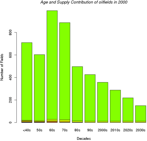
dimnames(mDiscoveryData )<- list(c("1+ mbpd","0.5-1.0 mbpd","0.3-0.5 mbpd","0.2-0.3 mbpd","0.1-.2 mbpd","0-0.1 mbpd"),c("Total production (mbpd)","<40s","50s","60s","70s","80s","90s","2000s","2010s","2020s", "2030s"))

head(mDiscoveryData)
barplot(mDiscoveryData[,-c(1)],xlab= "Decades", ylab= "Number of Fields", col=rainbow(20))
title(main = "Age and Supply Contribution of oilfields in 2000", font.main = 3)

par(mfrow= c(1,1), pch="+", lty= 1)
#
#   Total number of discovered field (affect the final URR)
#
nNumberOfFields <- 5500
#
#   Number of runs
#
M <- 100
vProduction <- matrix(0, nrow= 200, ncol= M)
vResults <- array(NA, dim= c(200, 6, M))
vMeanResults <- matrix(NA, nrow= 200, ncol= 6)
mAnnualVolumeDiscovery <- matrix(0, nrow= 200, ncol= M)
vWeight <- matrix(0, nrow= 1, ncol= M)
#
#   Main loop for the runs
#
vNumberOfFields= matrix(NA, nrow= M, ncol= 1)
nCentralNumberOfFields= sum(sum(mDiscoveryData[,2:ncol(mDiscoveryData)]));
for(m in 1:M) {
    nNumberOfFields <- floor(runif(1,nCentralNumberOfFields - 1000, nCentralNumberOfFields + 1000))
    vNumberOfFields[m] <- nNumberOfFields
    #   Simulate discovery data
    tabOilFieldData <- SimulateDiscoveryData(mDiscoveryData, nNumberOfFields)
    head(tabOilFieldData)
    mOilFieldsCurves <- matrix(0, nrow= 200, ncol= nNumberOfFields)
    #   
    #   The production staring year is the discovery date randomly shifted by 6-25 years
    #
    tabOilFieldData$yearstart <- tabOilFieldData$year + runif(nNumberOfFields,6,25)
    #tabOilFieldData$yearstart <- tabOilFieldData$yearstart - vPrice[floor(tabOilFieldData$yearstart)-1900];
    categoryGroup <- factor(tabOilFieldData$category)
    yearsFactor <- factor(1901:2100)
    decadesGroup <- factor(tabOilFieldData$decades)

    #volumes <- tapply(tabOilFieldData$URR, categoryGroup , sum)

    #barplot(volumes ,xlab= "Category", ylab= "Gb", col=rainbow(20))
    #volumes <- tapply(tabOilFieldData$URR, decadesGroup, sum)
    #barplot(volumes ,xlab= "Decades", ylab= "Gb", col=rainbow(20))
    #hist(tabOilFieldData$yearstart, seq(1901, 2050, 2), prob= F)
    #lines(density(tabOilFieldData$yearstart, bw= 3))
    #hist(tabOilFieldData$URR, seq(0, 120, 2), prob= F)
    #lines(density(tabOilFieldData$URR, bw= 3))
    idx <- 1:nNumberOfFields

    r <- runif(nNumberOfFields, 0.1, 0.2)
    #
    #   Compute each oilfield production curve
    #
    for(n in idx) {
        #
        #   Compute a standard curve (logistic or Verhulst) with a unity area
        #
        #v <- Verhulst(1:400, 200, tabOilFieldData$k[n], 1, tabOilFieldData$n[n])
        v <- Logistic(1:400, 200, tabOilFieldData$k[n], 1)
        #
        #   truncate production at the beginning ( ensure causality)
        #
        idx <- find(v[1:200] < r[n] * max(v))
        v[idx] <- 0
        idx <- find(v > 0)
        if (sum(v[idx]) > 0) {
            #
            #   scale the curve in order to match the URR
            #
            v= v / sum(v[idx]) * tabOilFieldData$URR[n];
            #v= v / mean(v[idx]) * tabOilFieldData$fieldoutput[n]; # alternative normalisation
      vCumulative <- cumsum(v)
      vCumulative[idx] <- (tabOilFieldData$URR[n] - vCumulative[idx]) / v[idx];
      idx2 <- find(vCumulative < 5)
      v[idx2] <- 0
            #
            #   Shift the curve at the staring year position
            #
            nLength= 201 -  floor(tabOilFieldData$yearstart[n]-1900);
            mOilFieldsCurves[floor(tabOilFieldData$yearstart[n]-1900):200,n] <- v[idx[1]:(idx[1]+nLength-1)]
      
        }
    }
   
    vTotalProduction <- rowSums(mOilFieldsCurves)
    #
    #   The average curve can use a weighted mean
    #
    vWeight[m] <- 1.0
    #vWeight[m] <- 1/mean((vTotalProduction[c(1:60, 82:105)] - vWorldProduction[c(1:60, 82:105)])^2)
    vWeight[m] <- 1/mean(c((vTotalProduction[1:60] - vWorldProduction[1:60])^2, (vASPORegularOil[4:8] - vTotalProduction[seq(85, 105, 5)])^2))
    vProduction[,m] <- vTotalProduction * vWeight[m]
    fSumWeight <- sum(vWeight[1:m]);
    tmp <- split(vProduction[,1:m] / fSumWeight, yearsFactor)
    means <- sapply(tmp, mean) * m
    stdev <- sqrt(sapply(tmp, var))
    n     <- sapply(tmp,length)
    ciw   <- stdev #qt(0.975, n) * stdev / sqrt(n)
    #
    #   Compute production curves by category
    #
    for(n in 1:6) {
     idx <- find(tabOilFieldData$category == n);
        if (length(idx) > 1) vResults[,n,m] <- rowSums(mOilFieldsCurves[,idx] * vWeight[m])
     else if (length(idx) > 0) vResults[,n,m] <- mOilFieldsCurves[,idx] * vWeight[m]
        tmp <- split(vResults[,n,1:m] / fSumWeight, yearsFactor)
        vMeanResults[,n] <- sapply(tmp, mean) * m
    }
    #vAnnualDiscovery <- tapply(tabOilFieldData$URR, factor(floor(tabOilFieldData$yearstart)), length)
    #vAnnualVolumeDiscovery <- tapply(tabOilFieldData$URR, factor(floor(tabOilFieldData$yearstart)), mean)
    #mAnnualVolumeDiscovery[,m] <- vAnnualVolumeDiscovery * vAnnualDiscovery * vWeight[m]
    #vMeanVolumeDiscovery <- rowSums(mAnnualVolumeDiscovery) / fSumWeight
    vTemp <- matrix(NA, nrow= 200, ncol= 1, , byrow= F)
    #vTemp[1:69] <- vWorldProduction[1:69]
    vTemp[seq(70, 105, 5)] <- vASPORegularOil
    matplot(x= yearsFactor, y= cbind(vMeanResults, cbind(vTotalProduction, vWorldProduction)), pch = 1:4, type = "l", add= F, ylab= "Gb/year", xlab= "")
    lines(x= seq(1970, 2005, 5), y= vASPORegularOil, add= T, type= "l", col= 2)
    text(x= 2070,y= means[130], "Total production (Excl. Synth. Oil, NGL)",col= 1,cex=.7);
    text(x= 2020,y= vMeanResults[120,1], "Cat. 1",col= 1,cex=.7);
    text(x= 2020,y= vMeanResults[120,2], "Cat. 2",col= 1,cex=.7);
    text(x= 2025,y= vMeanResults[120,3], "Cat. 3",col= 1,cex=.7);
    text(x= 2025,y= vMeanResults[120,4], "Cat. 4",col= 1,cex=.7);
    text(x= 2050,y= vMeanResults[150,5], "Cat. 5",col= 1,cex=.7);
    text(x= 2050,y= vMeanResults[150,6], "Cat. 6",col= 1,cex=.7);
    text(x= 1970,y= vWorldProduction[104], "Observed Production (All liquids)",col= 2,cex=.7);
    text(x= 1925, y= 29, sprintf("Iter= %d No of Fields= %d", m, nNumberOfFields), col= 2, cex= .9)
    text(x= 1915, y= 25, sprintf("URR= %6.3f Gb", sum(means)), col= 1, cex= .8)
    text(x= 1915, y= 24, sprintf("PO= %6.3f", 1900 + which.max(means)), col= 1, cex= .8)
    text(x= 1915, y= 23, sprintf("#Fields= %6.3f",sum(t(vWeight) * vNumberOfFields, na.rm= T) / sum(sum(vWeight, na.rm= T))), col= 1, cex= .8)
    plotCI(x=1901:2100, y=means, uiw=ciw, col="black", barcol="blue", add= T, ylab= "Gb/year")
   
}
lines(x=c(1901,2100), y=c(24.1,24.1), lty= 4)
text(x= 2075, y= 26, "ASPO estimate (24.1 Gb)", cex= 0.6)


{edit: 10/11/2005 correction of a few bugs}

[khebab]

Two results of simulation using the code above with two different scenarios for future discoveries.

Middle case:
Same amount of new discoveries fot the 90s up to the 2030s.



The full red line is the ASPO estimate for regular oil whereas the dashed red line is the all liquids oil production from BP. The horizontal dashed line is the ASPO estimate for the regular oil peak (24.1 Gb)

Low case:
The amount of new discoveries (small fields) diminishes gradually from the 80s



Both give the same estiamte for the regular oil peak date (2006). The estimated URR is around 2,200 Gb. The middle case scenario produces a bumpier curve post PO due to a larger production plateau from small fields (Category 6 fields). Even if we keep the same rate of discoveries of the 90s , it seems that the PO date won't be push back.

[WebHubbleTelescope]

Whenever I see a plot of the logistic curve, I always like to see the expression with values for the coefficients next to it. I believe that this consists of an overall scaling parameter, an exponential factor, and a time shift on the exponential for the simplest version.

[khebab]

Whenever I see a plot of the logistic curve, I always like to see the expression with values for the coefficients next to it. I believe that this consists of an overall scaling parameter, an exponential factor, and a time shift on the exponential for the simplest version.

In this case, it's a random sum of truncated logistic curves that can produce any kind of curves (even multimodal). Therefore, it's not a parametric model with a particular set of parameters.

[SilentE]

Even if we keep the same rate of discoveries of the 90s , it seems that the PO date won't be push back.

That's an artifact produced by your model assumptions. The lag between discovery and production means that the production curve for 2000-2010 was 99.99% determined by discoveries before 2000. Thus, changing discoveries after 2000 should have no discernible effect on a peak of 2006. Eyeballing the two curves, the differences only appear on the backslope of the curve, a few decades hence.

[Taskforce_Unity]

Your assumption is not correct SilentE. At the moment the average life after discovery when an oil field comes on-stream is approximately 4-6 years. Some oil fields come on-stream 2 years after they have been discovered!

[khebab]

That's an artifact produced by your model assumptions. The lag between discovery and production means that the production curve for 2000-2010 was 99.99% determined by discoveries before 2000. Thus, changing discoveries after 2000 should have no discernible effect on a peak of 2006. Eyeballing the two curves, the differences only appear on the backslope of the curve, a few decades hence.

I assumed a uniform distribution between 6 and 25 years to model the delay between time of discovery and time of production start. The economic context has obviously a huge impact on this time lag but it's a challenge to derive a statistical relationship oil price, available capital and decision to invest in new production.

Your assumption is not correct SilentE. At the moment the average life after discovery when an oil field comes on-stream is approximately 4-6 years. Some oil fields come on-stream 2 years after they have been discovered!

I didn't know that it could be as fast as two years! I assume it must depends on the size of the field and its location (offshore fields must take longer). Do you have any data on that?