The Fake Fire Brigade – How Can Renewable Sources Support Our Current Energy Delivery Expectations?

In this post, we try to develop a systemic picture of electricity, using some of our European models.  We will put a specific emphasis on wind power, as wind is seen as the single most relevant renewable source, and many plans involve a share of approximately 20%-30% of total power consumption within the next 10-20 years, and even higher in the longer term.

In the last and final post, which can be expected to follow approximately next week, we will cover all technologies we consider relevant one by one – in all fields like electricity generation, storage, distribution and demand management. But before diving into this week’s post, we would like to answer a few questions that came up 10 days ago.

Industrial energy prices in Europe

One of the arguments we heard when looking at “bearable” electricity prices was that in Europe those prices are much higher. This is not correct for industrial energy uses. The data available is grossly misleading, as it posts public rates for relatively small users (for industrial customers). All the countries that still have a significant heavy industrial electricity use provide energy at prices for large industries that are relatively comparable to the United States.

Let us use Germany, the largest European economy, as an example. According to the German statistics authorities, the pretax electricity cost in 2007 was at 10.9 Euro cents per kWh on average (this is the latest data available, but only in German). There have been no significant changes in electricity price in Germany since, except for higher contributions towards feed-in tariffs for renewables, which were partly offset by to lower prices due to excess capacity – a product of the recession. For industrial and commercial customers, cost per kWh was 8.6 € cents on average. Large industrial users, of which the most energy-hungry are exempt from supporting feed-in-tariffs for renewable energy, paid between 5-7 € cents (see: Bedeutung des Strompreises für den Erhalt und die Entwicklung stromintensiver Industrien in Deutschland).

When applying purchasing power parity exchange rates (which is what really matters and fluctuates much less than average exchange rates in markets) of approximately 1.15 dollar cents per Euro, this translates to 12.5 $ cents per kWh on average for all customers, with a slightly different distribution between private households and industrial customers when compared to the U.S.

At the same time, what you see in Germany for example is that more and more heavy industrial electricity users disappear from the country with rising cost of electricity. Primary aluminum and secondary steel production are mostly gone by now, and automobile manufacturers import a larger and larger share of their components from low wage and low energy cost countries. This is a relatively clear consequence of higher energy cost.  So even in Europe, industrial users still pay electricity prices that are within the “green” to “yellow” range of our table, but already there is huge pressure to avoid that cost.

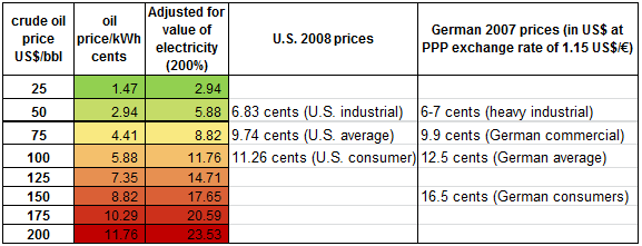Table 1 – electricity cost limits (with U.S. and German prices)

So overall, industrial prices are very comparable between Europe and the U.S., but in both places they are already high compared to China, for example.

The cost share of energy – societal EROI

Another aspect that is being discussed repeatedly is that energy currently has a share of “only” 5-10% depending on country for OECD countries) of total GDP, and if that share grows or even doubles, this wouldn’t affect things so much. Unfortunately, this view is based on a significant misconception, as it ignores the special role energy plays in our human ecosystem. The cost share for generating, distributing and enhancing energy is a very good proxy for societal EROI, i.e. tells us how much we can get out from our energy extraction efforts. We will not go into too much detail here, as this would justify another 10,000 words, but a brief introduction might be advised.

In a society where energy cost is 5% of GDP, this means that for each “unit” of effort that goes into the generation of energy, 19 units of “benefits” in the form of consumption and investment can be extracted for society. If that share doubles to 10% of GDP, we suddenly can only extract 9 units of benefits per unit of used energy. We can look at this in two ways: first, in the production system, then in the consumption system for individuals.

Important: the role of humans in advanced (and parts of emerging) economies is no longer the one applying physical work, but it is directed at the management of energy extraction and its application towards a use that is considered beneficial – ranging from food to buildings to plastic toys and cruises in the Caribbean.

If we analyze the manufacturing of goods, with the exception of a few novelty and luxury items, their price is very much driven by energy cost, either the cost of human labor (expensive to very expensive energy) or the cost of other energy applied. This energy includes not just the energy used to produce a good, but equally the energy used in the extraction, refining and manufacturing of raw and intermediate materials, in transportation, and in buildings and infrastructure used. The latter is “past energy” that might have come at a different price, but since we theoretically have to rebuild the infrastructure over time to maintain our ability to continue into the future, this is only marginally important.

Food is a very good example of the importance of energy costs required in production: producing and processing today’s food consumes much more (fossil) energy than it generates in the form of calories that get consumed in the final meal. From 2000 to 2010, the food price index (World Food Situation) has grown by a factor of almost two (it even went above that in 2008), which is very much in line with the development of average energy prices (oil and natural gas were the key price drivers). Commodities show an almost identical pattern (Table 1a. Indices of Primary Commodity Prices, 1999-2010).

So if we look at a society where energy cost increases from 5 to 10% of total, it is likely that very soon, the share of food costs will grow comparably. And the same is true for almost everything we consume that contains significant amounts of embodied energy, but consequences often aren’t visible so quickly if, as – for example – factories built with lower cost energy are still producing most of the output. But when a new factory has to be built, this will immediately be reflected in the price of the final good.

Energy conservation – the biggest resource (?)

We have been repeatedly called out for not including energy conversation in our posts, so we decided to include a brief “why” at this point. The first and most important reason is that energy conservation doesn’t significantly change the dynamics of electricity delivery systems. Irrespective of total level of consumption, overall usage patterns don’t change significantly, and so neither do the problems and issues of generating reliable electricity for a society.

Conservation will happen anyway with higher energy prices, as we can see in Europe, where energy prices on average are approximately 1.5 to 2 times higher than in the United States. From there, we see that rising prices drive consumption down, influenced by three factors:

• Countries give up on highly energy intensive activities and (as long as they can find places like China or Norway with cheap energy) outsource them
• More energy-saving technology gets introduced and used, for example fuel-efficient cars. My own German car gets 40 mpg (on Diesel, equivalent to about 35mpg on gasoline). A significant portion of those energy savings come from higher cost of equipment, and also slightly higher energy consumption in its production (often from cheaper energy sources)
• Less overall consumption

In industrialized Europe, this has led to a reduction of an economy’s energy intensity by about 20% over the course of the past 20 years, but our models estimate that total energy efficiency gains that factor in “energy used elsewhere” (particularly in China) reduces this gain to about 5-10% – or in other words: net energy savings are far lower than actual local consumption data suggests.

Equally, total conservation benefits are often overstated. Light bulbs are a very good example. While modern fluorescent energy saving lights consume only about 1/3 of the energy a traditional bulb uses, that isn’t the full picture. First of all, more energy is used to design, manufacture, transport and recycle the modern bulb, which essentially is a little computer. This might not matter for bulbs that get heavily used, but for the not too few instances where the bulb gets thrown away (often with the lamp) before its now extremely long life has expired (6000 hours totals to 33 years for lights that are on ½ hour a day on average), it does. What matters more is that all those benefits only apply to the most expensive of CFL lamps, the cheaper ones purchased for 2-5 dollars are often much less efficient or last much less long.

Then, when looking at the traditional indoor use in moderate climates, at least 65-75% of the use of light bulbs occurs during heating periods, when heating is required. During these times, the “loss” from traditional bulbs in the form of heat gets fully added to the ambient temperature of that room, thus reducing the need of additional space heat. When all these aspects are factored in, the theoretical 65-70% advantage of new lighting technologies is reduced significantly less (see for example Benchmarking of energy savings associated with energy efficient lighting in houses).

This isn’t to say that we shouldn’t try to conserve energy – we should – but in the picture we are trying to draw, it doesn’t make that much of a difference as long as we don’t reduce our standard of living, and – most importantly: the level of energy consumption, as mentioned above, doesn’t matter too much when it comes to securing a stable electricity delivery pattern, unless we go so low that we can use reliable reservoir/dam based hydropower as the main source. That would clearly be Utopia.

A model case to work with – wind power in Europe

Throughout this post, we would like to stick to a simulation of future energy systems to explain some of the problems we see coming our way. The data introduced below will accompany us throughout the entire post, so it might make sense to spend some time explaining it.

To understand a future energy delivery system with large inputs of renewables, we use significantly sized wind power, in an integrated model grid of three powerful wind locations, Spain, Britain and Denmark.

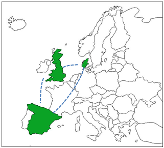Figure 1 – Simulated European wind delivery system with connections

Spain (blue in Fig 2 and 3) data is taken from actual production numbers available in 20 minute intervals (Detalle de la estructura de generación en tiempo real). The country currently produces about 14.5% of its total electricity with wind (The status of wind energy in 2009 By GWEC). Most importantly, Spain is a very favorable place for high wind power penetration, as it is surrounded by oceans and – thanks to its location, exposed to two different weather systems, one influenced by Atlantic, the other by Mediterranean winds. This makes its total wind output profile the most balanced one we know of.

The green line shows the simulated wind output for England Scotland and Wales (calculated from hourly weather data across the country). To make things comparable, Britain’s output is normalized to match the Spanish total annual output. This represents a wind market share of approximately 11.5% in Britain.

The green curve uses real wind output data from Denmark, which we have equally normalized to the same size of the Spanish output. This should quite well represent the entire geographical area (including Northern Germany, for which no hourly data is available).

In our model, all three “systems” produce the same amount of electricity per annum, about 36.2 TWh. The red line represents the average hourly output of all three areas, and the horizontal light blue line the standard average output required all year long to match demand. Note: We used a straight line to simplify the picture, we could equally have included the normalized consumption of all areas. As we have tested all our models against both this straight line and against real consumption without significant differences for wind power, we use the simpler model here.

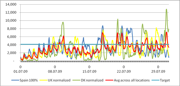Figure 2 – wind simulation for Europe: July 2009 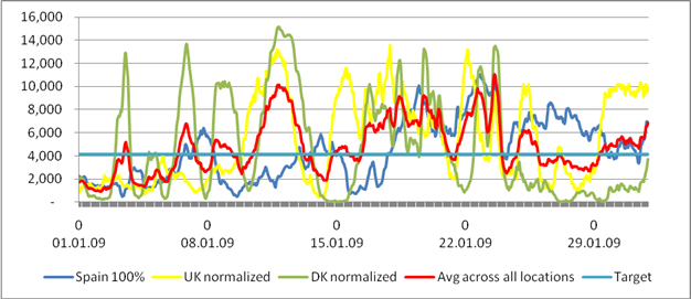Figure 3 – wind simulation for Europe: January 2009

Above, we have selected two typical months for the year 2009 – but others show the exact same patterns. The only visible difference is that on average, wind output in winter is slightly higher than it is in summer. But in both months, the average output of those three areas ranges from very low to a multiple of the expected target, and each area by itself shows even stronger fluctuations, as would be expected.

Below, we want to see what this translates to. Note: We use Europe as an example because we have so far found no reliable data for the U.S., but preliminary research confirms that the difference between the two continents is not significant. We are happy to re-run our models if someone is able to provide us with real (not modified) U.S. wind data for all the key regions suitable for wind power in the U.S.

Myth #1: The wind always blows somewhere

This is one of the common hypotheses stated by proponents of long range super-grids. A number of studies have looked at this issue. Among them is one that gets cited in almost every paper about Europe (Equalizing Effects of the Wind Energy Production in Northern Europe Determined from Reanalysis Data). It has a methodological flaw in that it doesn’t differentiate between areas suitable for wind and others where wind doesn’t blow strong enough, but this detail doesn’t matter. It shows a correlation coefficient of wind patterns across all of Europe is between -0.2 and 1, with most correlation coefficients being between 0 and 1.

We now have to get a little mathematical. A correlation coefficient of 1 says that things are strictly in synch, e.g. for wind it would tell us that when it blows in one place, it also blows in the other with the same or with proportional strength (please see the first example in Table 2 for this).

A correlation coefficient of -1 tells us that two values are strictly inversely related, so when the wind blows in one place, it doesn’t blow in the other, and vice versa (example 2 in Table 2). A correlation coefficient of 0 simply says that there is NO correlation between the two sets of values, or in other words: if the wind doesn’t blow in one area, it might or might not blow in the other (example three in Table 2).

Table 2 – samples for correlation coefficients

So obviously, if wind is correlated, it isn’t good for sharing. Ideally, wind outputs in regions sharing wind power would be negatively correlated (-1 or close).  If correlation coefficients are around 0, we simply can’t tell, i.e. there will be days when the wind blows strongly in both places, days where it doesn’t blow in both and days where they complement each other (the set of random values in the third column of Table 2 shows exactly that).

Going back to our initial example: the total hourly outputs for Spain, Britain and Denmark show correlation coefficients of 0.08 (Spain and DK), 0.09 (Spain and the UK), and 0.32 (UK and Denmark). This is pretty much in the lower range of the previously quoted study, so our three areas are probably good ones to realistically try the concept of sharing across large areas.

This mathematical reality, combined with Fig 2 and 3 very quickly discourages the belief that “the wind always blows somewhere.” Well, we don’t want to say that there isn’t a tiny bit of wind that always blows somewhere, but not to an appreciable degree.

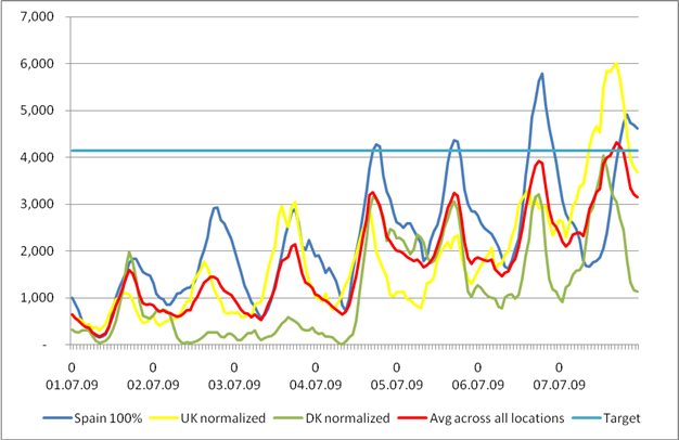Figure 4 – First week of July – 3 Sites with correlation coefficients of 0.08, 0.09 and 0.32

The above week in July shows, how wrong that assumption can go. The lowest average electricity output in all three sites in 2009 is 173 MW (4.1% of target) in one hour. Throughout the year, this situation comes back repeatedly, while equally, there are hours where the maximum output amounts to 11.6 GW (280% of target output).

This translates to a simple reality: during those hours of low output, power has to come from other available capacity, demand has to be drastically reduced, or the grid will break down.

The characteristics of generation technologies

In order to not get bogged down in mixing everything with everything and ending up with hundreds of possibly unrealistic assumptions, we have to look at individual technologies separately in order to judge their ability to contribute to a stable electricity delivery system and to see whether they – as combinations, will be helpful.

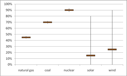Figure 5 – uncontrolled variability of multiple sources (aggregate view)

Figure 5 shows a problem we will analyze in more depth further down. For an aggregate of stock driven generation tech­nologies (like all natural gas, coal and nuclear in any given country), unplanned variability is close to zero (fluctuations come from unexpected outages of single plants), while for solar and wind, all outputs between 0% and 100% of nameplate capacity are possible and realistic. Additionally, these sources have a very low average output relative to their maximum capacity, probably between 11-16% for solar in aggregate for a country, and about 15-26% for wind (in aggregate, not for individual turbines). This is one of the biggest challenges with renewable technologies, that they only produce a low average of their maximum capacity. This means two things: a lot of generating capacity is required to get the same average output when compared to other sources, and inversely, when production is good, a lot of power becomes available at once.

In our first post, we quickly reviewed the fact that renewable energy sources are growing at a slower pace than traditional fossil fuels. Often, this gets countered with the impressive growth rates of renewable technologies, which then get extrapolated into the future. Unfortunately, not everything continues to grow exponentially, particularly if the integration into current delivery systems is so difficult.

But one other thing that is often misleading is the fact that “installed capacity” is counted. This has nothing to do with produced electricity, but with the peak output a technology can accomplish. While fossil fuel driven power plants can be run close to 100% of capacity based on human decisions, renewable sources are typically operating at much lower rates. On a global level, total achieved outputs of wind are around 20% of possible output per annum, for solar around 12%. So while we may count on natural gas or coal with an availability of more than 90% of capacity (even if we don’t use it all the time), renewables can only be accounted for at a fraction of their official nameplate capacity.

Table 3 – capacity factors and controllability of sources

Now in order to understand what can be combined and what not, we have conducted an analysis of what energy sources are “compatible” with one another to understand which combinations can ultimately be beneficial.  Our summarized results:

Combinations only make sense to be reviewed when they have a generally complementary profile. Let’s use an example: Solar and Wind. While we have some positive correlation – often sunny days are less windy, we also see the opposite – very sunny days where strong winds blow – which further improves PV output (panel temperature is negatively correlated with electricity production, so a cooling breeze increases PV efficiency). Equally, we can expect that during snowy wintery late afternoons with cold temperatures both wind and sun don’t deliver much output. That makes those two technologies not truly suitable to supplement each other, because we can predict with 100% certainty that they will create dangerous situations for grid stability on a regular basis.

In Table 4 below, we provide an overview of the characteristics of each energy source and its suitability with others. This will be further analyzed in more detail in individual paragraphs for each source, but this should give a first overview of what is compatible and what isn’t. The first row shows their key characteristics (load type, predictability), the cross matrix looks at their compatibility. This is a brief overview, in our review of individual technologies, we will look at this in more detail.

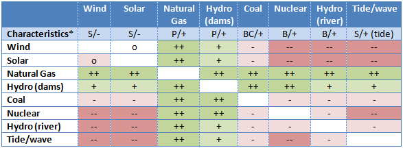Table 4 – Characteristics and cross-compatibility of generation sources: Legend: S=stochastic relative to demand, B=Base, C=Load Following, P=Peak, Predictability: + good, o=average, -=low

Ultimately, the best way to understand energy sources is to review their ability to fit the human demand system, which is – and always will be – relatively steady over long periods, and with specific fluctuations related to days, weekdays/weekends and seasons. In the end, we will try to analyze each source and each possible combination in order to understand its capabilities to work together with others, but first, we want to look at a number of large scale “solutions”.

Myth #2: Long range HVDC transmission solves problems

One of the cornerstones of future energy concepts is the introduction of long range transmission for multiple purposes. First, this should help share renewable outputs when they differ between multiple regions, and second, provide access to flexible resources (like hydropower). We would like to analyze the sharing across regions a little more closely.

Unfortunately, since there aren’t any negatively correlated sources within reach, there might be some benefit from sharing, but that isn’t as big as one might expect. Let’s look at the three wind locations (Spain, England, Denmark) a little more carefully for that. Upon closer analysis, it becomes clear that sharing excess renewable energy only makes sense under very specific circumstances. We conducted an analysis as to how often this positive effect would be seen, and how much (or how little) could be shared in those situations. Important: sharing only works when one location has too much and another one has too little – if all have too little or too much, it makes no more sense to transport energy. As Table 5 shows, a “sharing” situation occurs in 42.2% of the cases. With this, about 10% of total wind output can be shared across the three regions, filling about one third of the (mostly smaller) gaps.

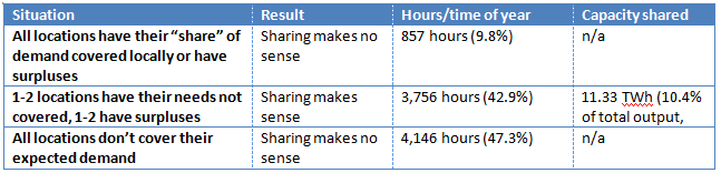Table 5 – sharing situations

Unfortunately, the hours where sharing is possible mostly relate to relatively “uncritical” situations in the “middle”. The largest amount shared in any one direction is slightly above 4.2 GW. So in order to build the necessary “power highways”, three HVDC connections (see Fig 1) with 4.2 GW capacity would be required to explore the benefit, with a triangle connecting Denmark and Northern Germany, Britain and Spain. Due to the fact that sharing only happens a fraction of the time and often for much smaller amounts, the capacity of these three lines would be utilized at only 10%, which makes establishing these HVDC lines quite uneconomical.

As shown below in Figure 6 for July 2009, this approach doesn’t do much for the most critical situations, neither where wind produces too little output in all three areas, nor in those moments where it is too strong everywhere.

Figure 6 – Long range HVDC potential in 3-region analysis

An estimate for the cost of three 4 GW cables forming a triangle with segments of 700, 1000 and 2000 each between Britain, Spain and Denmark/Northern Germany (Figure 1) arrives at a ballpark of roughly $10-12bn. If we assume an investment of $10bn, a life expectancy of 30 years, an interest rate of 6% (which is rather low and only slightly above 30 year bond interest rates) and maintenance cost of 1% per annum, the cost for each wind kWh usefully transmitted between the three countries would be more than 7 cents, not including line losses and operating energy for the heavily underutilized HVDC equipment (as stated above, utilization would be at approximately 10% of capacity). And, which is important, we haven’t really solved the most relevant problems yet – underperforming wind farms and high surpluses in all three locations simultaneously.

So for a very large investment, we ultimately get very little in return; and in all those situations (almost 50% of the time) when all three regions don’t have enough wind, it doesn’t help at all. For those, we need other solutions, once again.

Note: As stated before, in this model we used demand as a steady line to make it easier to understand and compare. When using demand patterns instead, the end result is almost exactly the same. Critics of our approach will now say that we have to introduce storage to deal with the other, uncovered parts. Let’s see how that works.

Myth #3: Storage will fill the gap

Now that we have seen that long range sharing via supergrids likely won’t deal with situations when all locations produce way too little or way too much, we have to look at storage. The above example, where 3 regions have about 12-15% wind power in their energy mix, might serve as a good example.  If we start in early January, the cumulative gap that builds up from January 1 to January 6 (across all three areas) is approximately 740 GWh. Within those six days, all three regions underperform most of the time. So during this short period of time, the 50 GWe (nameplate capacity) of installed wind capacity would accumulate a deficit worth almost 15 hours of operation at full power, and 60 hours at the expected average load factor (25%)

That was just for starters. Even when sharing across all three areas, the highest cumulative gap (compared to average output) amounts to 6.75 TWh in 2009, equal to 22.5 days of average wind output. Without sharing, the maximum cumulative gap was 34.5 days in Spain, 24 days in the UK and 20 days in Denmark. This result again shows how little the supergrid can actually contribute.

In our first post, we have shown this exact same problem for a simulation for the UK, we include the same graph again as a reminder:

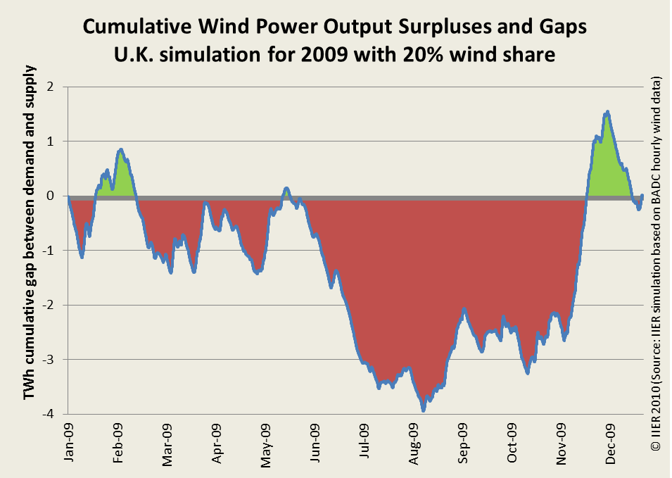Figure 7 – Britain long term surpluses and gaps against power demand

The reason for this lies in seasonality and heavy arbitrary month-to-month fluctuations. Below is a graph that shows the average daily production in the three European regions we analyzed.

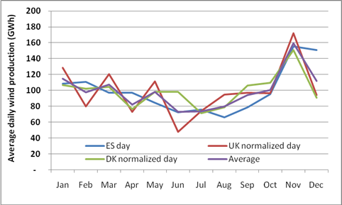Figure 8 – Monthly fluctuations.

November 2009, for example, forms an extreme case. In this month, all three sites ON AVERAGE produced 159% of October and 142% of December wind output. Seasonally, things look even worse; November 2009 produced 228% of June output. Average daily output during the strongest three months in 2009 (November to January) was 70% above that of the weakest three months (June to August).

Some people have dismissed this approach of looking at long term gaps, but the problem is grave: of the expected outputs, a significant portion has to be shifted in time, intra-seasonally, or across seasons. This requires either other sources that are flexible enough (see the paragraph below) – or storage. In this section, we want to think about using storage to make up for those large amounts of surpluses and gaps.

For a mental exercise, let’s assume that we only have wind power and a storage technology: in order to match one MW of wind nameplate capacity with enough storage to not lose too much of the excess production at high wind time and to be able to bridge all the gaps, we would have to provide capacity worth approximately 20 days of average wind output, which – with a capacity factor of 25% – totals to 120 MWh of storage capacity for each MW of wind power production (6 MWh per day x 20 days). In the comments to our last post, someone pointed out a solution for pumped storage in oceans (Large-scale electricity storage) with a capacity of 20 GWh. We will look at this type of storage in the next post when reviewing individual technologies, but for now, let’s assume this solution is feasible. This huge (10×6 km/6×4 miles) artificial island which will cost at least $4-5bn to build according to our estimates (derived from the amount of material required and other sources on building artificial islands like it was done in Dubai) would support not more than 167MW of wind nameplate capacity, which is the size of one average offshore wind park costing about $650m. This simply doesn’t work – the storage technology costs 8 times what the generation technology costs. Another example: pumped storage in favorable geographical locations (not the power island mentioned above), costs about $100m per GWh of storage capacity. One GWh would be able to support a mere 8.3 MWe of installed wind capacity, which costs approximately $20m to install. So for each dollar spent on wind, 5 dollars would have to be spent on pumped storage. So even if we only tried to store 20% of it, doubling the investment cost doesn’t sound like a good deal. And – as we will see later, pumped storage – when available – is among the cheaper and most durable options.

The reason for this cost problem has to do with the characteristics of current fuels: all successful uses of energy “stocks” – with the exception of hydropower, which instead uses large natural water bodies and gravity – are based on the irreversible destruction or reduction of complex molecules or atoms, where the energy is stored in the form of intra-atomic or molecular particle bonds and then released. Mostly, they burn (coal, oil, gas, but equally wood), and in the case of nuclear power, the kinetic energy from the release of neutrons and photons that get split off. All these processes increase entropy and convert a high quality molecule or atom into something simpler and more abundant.

Storage instead operates with a reversible process. In many cases it is simply physical, like in heat, cold, pressure or altitude difference, or – with batteries – by chemical reactions that are based on moving molecules between anode and cathode. Other than that there are a number of chemical batteries based on relatively single molecule oxidations, a principle used in single-use batteries or with hydrogen, where H and oxygen atoms react to water, releasing energy. Unfortunately, these oxidation processes have a relatively low round-trip efficiency.

Most “efficient” storage technologies suffer from another significant problem: one of energy density. While our mainstream chemical “destructive” processes release large amounts of energy per volumetric/weight unit, none of the physical or simple chemical processes can ever come close, and never will, despite all improvements in their technology development.

Table 6 shows an overview of “storage” technologies, including those where nature did the storing for us through millions of years using pressure and heat. It also shows the price per “kWh” of storage capacity. For all “natural” resources, we don’t have to pay that price, we only pay the cost of extraction.

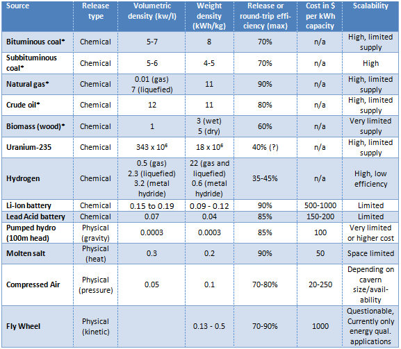Table 6 – “storage” solutions (*non-active energy storage) – preliminary, still under research

Figure 9 shows this very illustratively – the energy density of all storage technologies is a fraction of the content per volume or weight unit in fossil fuel stocks. And the only option with halfway meaningful weight density (hydrogen) has a very low round-trip efficiency and an unfavorable volumetric profile.

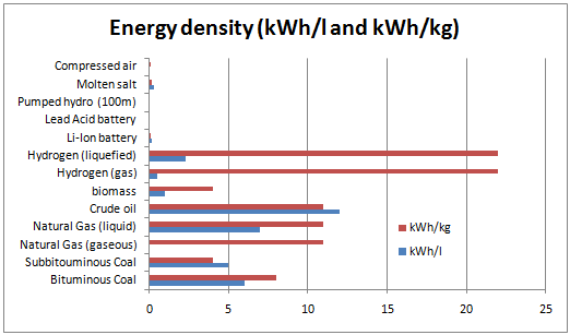Figure 9 – Energy density of primary energy sources and storage

So ultimately, storage isn’t capable of dealing with the big shifts. It is capable of handling intra-day imbalances, maybe weekends and holidays and – for example with pumped hydro – works great to help balance nights and days with less flexible sources like coal or nuclear, but not in those longer term situations we will experience with large scale wind or solar power.

Myth #4: Demand management (smart grids) can solve the problem

We discussed demand management in earlier posts, and in response to our previous installment (#3), we had a number of comments indicating that more actively managing demand could be a good way of dealing with ups and downs in electricity supply.

Unfortunately, this offers the same challenges as storage does. In a world with renewables having a high share, we no longer talk about regular patterns of supply and demand where nights and days show a certain mismatch, but we talk about over- and underproduction for days, weeks and months. Dimming the lights in office buildings, or storing heat and cold no longer work in this case. Only a small fraction of surpluses and deficits can be shifted within 24 hours, the problem basically is the same as with storage – we are talking about long term gaps. Only if a technology was capable to move a significant amount of demand – for example – from October to November (in 2009), it would create benefits to solve the problem we are discussing here.

Still, we briefly want to look into “smart grids” and what they are supposed to do. There are multiple forms of what is considered “smart”. Here is a brief overview:

In a passive, simple form, so called “smart meters” are supposed to provide information and feedback to customers, mostly about the current price of electricity. That way, market incentives should be created to use less electricity during peak times and shift some demand to times with higher availability. This already happens today with night/weekend and day tariffs, and with industrial and commercial customers, where large devices mostly get turned on during low cost times (entire operations plans in industrial companies get organized around lower electricity rates). On industrial and commercial level, a significant amount has already been accomplished when it comes to smoothing out day and night peaks and lows based on demand management, but households have not really been explored so far, except for different day and night/weekend rates. With smart meters, there is a hope that customers might receive sufficient information about their energy options and thus change their usage patterns. A number of pilot projects have been undertaken so far to understand the implications of this approach, mainly in Germany and the Netherlands. Results are disappointing. We are happy to share some links (all in German) that point to recent studies, but there are two outcomes, in general. First of all, for average households, the expected savings are not able to recover the additional cost of the technology (two-way communications between utility and end user, new meters, software, operations). For Germany, savings are estimated at around 10-40 Euros per annum and household, with initial setup cost around 50-100 Euros and annual operations cost of at least 50 Euros. Second, a Dutch study shows that very conscious users participating in a study might accomplish up to 8% savings in their electricity consumption initially, but that this effect wears off quickly. Other studies confirm those results. The reason seems relatively clear: with the tight time schedules most people have, monitoring electricity to find the best times to run their laundry might only be something for very conscious citizens, but not something for the average person. And large consumers, commercial and industrial users, are already participating in those schemes.

This becomes even more challenging as the key difference compared to today would be that with renewables, these patterns become absolutely unpredictable. It is possible that suddenly, during the night, there isn’t enough power, and it is equally feasible that there is way too much during previous daytime peak hours. This would constantly ask for a change of life routines, something humans are notoriously bad at.

So if we are not ready and able to “manually” steer electricity demand, this asks for those more advanced form of smart grids, which are capable of – without user intervention – turning devices on and off. Laundry could be postponed automatically until low cost electricity is available, a freezer could be turned off for a while and still hold its temperature, and so could heating and cooling appliances, or lights (in office buildings) could be dimmed down. In this case, routines of users might not really be affected, as long as we don’t turn off the TV set during that important baseball game.

Now, there are two caveats: first, again the fact that we might have a “low supply” situation for much more than just a few hours, but instead for days or weeks. Or inversely, there might be the same with oversupply, it might last much longer than any use could consume. So while we might be able to turn an air conditioner off for a few minutes, or even for a few hours if it operates with ice storage, we can’t do that for a couple of days without making life unbearable in Texas, Nevada or Southern California, for example. The second problem is equally big: this approach does require a lot of investment into new devices, as it will be impossible to retrofit most household appliances, particularly those with electronics, which don’t take a simple power cut all too well. So a large amount of investments into new appliances would be required, exactly at a time when recessions and other limits make it hard for people to pay their normal bills. On top of that, replacing still working equipment with new, “smarter” devices also incurs significant energy consumption, which first has to be recovered, both economically and energetically.

The last aspect of smart grids is the idea to introduce electric vehicles into the grid and use connected vehicles as an “extended storage device” for surplus electricity, and as buffer for power gaps. As we already mentioned in our initial “fake fire brigade” post, gaps and surpluses are so grossly disproportional compared to what an ELV fleet could offer, that using expensive Li-Ion batteries which only survive half a car’s life span for storing regular energy seems like a very silly thing to do, as it further shortens the life expectancy of this expensive piece of equipment, without making a significant dent into the imbalances in the grid. A preliminary calculation we performed shows that it would cost approximately 70-80 cents to store one kWh of electricity in a high-tech ELV battery. Not exactly a bargain.

So again here – as with the other things – smart grids and other demand management efforts don’t really seem to offer what is required to manage the instability of future energy sources, they mostly add cost and complexity.

Myth #5: Together everything will work out

After introducing supergrids, storage and demand management, the vast majority of gaps and surpluses from wind farms still aren’t dealt with, because their impact is just too small to significantly influence the situation. If suddenly all wind farms in a country produce 3 or 4 times as much as their expected average, how should anything be able to pick up that much power? In a world with 30% wind, this easily amounts to more than 100% of total consumption – even with 20-25% wind coverage, wind sometimes produces more than total demand during low times. And in case all of them fall down to almost zero for a week or more, how should any of the three solutions be able to fill a 30% gap in production?

To better understand this situation, let’s look at some specific days in 2009, for example January 1-6 in our model of Spain, Britain and Denmark. By this day, all meaningfully available storage will be empty, sharing doesn’t provide any benefits, but wind power output is still 8 TW short of what is expected. On July 1^st, we have the exact same situation, but almost 12 TW are missing, while all storage has long been emptied. The only thing that helps to fill that gap is flexible generation capacity that has to sit idle until that day comes.

Today, this is done mostly by hydropower (from storage behind dams) and natural gas, which can be turned on when such a situation occurs, and there is no reason to believe that this wouldn’t be the sources of choice for the future. However, there is a caveat – availability for a world with 20, 30 or even 50% of renewable power.

Hydropower can only support a fraction of what is required and has only limited expansion potential (please equally see detailed technology reviews in the next and final post), plus it is equally seasonal – strong in winter and spring, but rather weak in summer and fall (in the northern hemisphere). So unless a country has a beneficial topography, hydropower potential is simply limited.

So ultimately, we are stuck with natural gas. Modern natural gas power plants have a life expectancy of approximately 100,000 hours (11 years at full time operations) OR 3000 starts (one start puts stress on the equipment worth 333 hours of operations, please see Lifetime Extension for SIEMENS Gas Turbines). With maintenance, this can be extended by about 50-60%. If we were to support large wind power with natural gas, we will see a much lower capacity utilization of a required much larger fleet of standby gas power plants, but many starts and stops. So in the future, we can’t just plan to continue using already existing power plants, but instead that capacity has to be specifically (re)built for the type of situations that keep coming back regularly, month after month, year after year.

Since storage and sharing won’t allow us to have secure stable electricity, but instead would leave us with heavy fluctuations (and thus blackouts, if unmanaged) as soon as we introduce wind at a significant share (which might be as low as roughly 10% across entire larger grid areas, not just in small isolated situations like Denmark). With hydro not truly scalable, the only remaining technologies are fossil fuels, mainly natural gas, which for its flexibility and relatively low price work best. Or in other words: in a world without abundant natural gas (or an equivalent flexible stock), large market shares of wind simply won’t work.

A simple conclusion can be drawn from this analysis: combining all three options – using stocks, sharing across geographical areas and large size storage – doesn’t create more benefit than balancing with natural gas alone does, and without those stocks, it definitely doesn’t solve the problem of variability in outputs. The contrary is true: a combination adds cost to the system, and creates complexity. At a certain point, because all those extra technologies use fossil fuels in their production, installation and maintenance, their use might not even reduce overall carbon emissions. Even when combining all of it, it  doesn’t mean that we need less gas power plants, it simply pushes utilization of those plants down, because they still have to be kept available for those unpredictable but absolutely unavoidable events when everything else fails to deliver.

To quantify this risk of failure: even across all three regions (England, Spain, Denmark), there were 77 scattered events in 2009 where SHARED wind produced less than 20% of expected average output, and 9 events where it produced less than 10% of what was expected. For all these situations, stock based capacity needed to be available (sitting mostly idle during other times).

Why do other studies come to different conclusions?

The assumption when we started our research was that everything had been resolved and clarified regarding the intermittence of wind power and the risks associated to it. Numerous studies and concept papers seemingly have answered the questions we asked ourselves, coming to the conclusions that there will be no insurmountable hurdle to establishing a large (30-50%) share of wind power in electricity systems. Over time, we found out that there are a number of flaws in all those papers:

• Not enough analysis of the detail: by simply using statistical methods, the risk arising from RARE BUT CERTAIN supply situations in electricity grids often get overlooked, only full simulations looking at exactly those reveal the true problem. And if those “rare” events occur 60 times every year, it means that there will be an unavoidable blackout more than once a week on average.
• Focus on short term fluctuations instead of longer-term variability: one of the most important mistakes of most studies is to look at “unpredicted” variability of wind power alone. This deals with the question of how much reserve capacity has to be held available to manage unexpected gaps in wind production. Given the improvement in weather predictions, this problem has become smaller over the past years, i.e. reserve requirements to match short-term shortfalls in wind output have become smaller despite growing capacity. However, what these studies do not deal with is the shortfall relative to demand, which can mean that – in a situation with a 30% wind market share – there will be times where 30% of expected supply has to come from other sources, and equally distressing, that wind power plants occasionally produce more than 100% of demand.
• Belief in combinations: often, analysis of certain technologies does not carefully study other technologies they consider relevant as supplements in sufficient detail, which gets authors to the (false) conclusions that their problems will be solved by someone else. This is true when suddenly biomass or waste burning should make up for gaps in production, or pumped storage should be scaled up to solve the problem. Only a careful analysis of all participating systems would reveal this misunderstanding, but specialization in one field often makes recognition impossible.

Truth #1: There is no stable electricity without stocks

We have now used sharing via supergrids, storage, and demand management, and still haven’t even gotten close to balancing the variability of wind power. Our readers will now say – and correctly so – that it makes no sense to try to manage those long-term fluctuations with storage, but that we should instead use other generation technologies to make things work. That makes perfect sense, and is what happens today – fluctuations in wind power get balanced out by cranking other sources up or down. All those “balancers” are stock-driven sources (see our previous post for more detail on this). As we will see later, the best ones currently available, after fuel oil has become too expensive, are hydropower (from reservoirs behind dams) and natural gas, which are flexible and economical to compensate situations with high fluctuations. But why, if those offer a meaningful solution, are we spending so much time and money on storage and supergrids?

So the bottom line is as simple as that: wind and other stochastic resources are unable to deliver electricity 24/7 on 365 days without scalable stock based generation technologies that are able to match almost 100% of expected power outputs from those renewables. Storage, sharing or demand management won’t significantly help to deal neither with surpluses nor gaps.

Of all flexible stocks, natural gas is the only one that is currently available, affordable and scalable, and there is no reason to believe that this will change anytime soon. All other sources are not flexible, not scalable, or too expensive to play the same role. But even if it won’t be natural gas in the future, it will have to be a high energy density stock and its generation capacity needs to sit idle and wait for gaps to be filled. What this approach still doesn’t solve is the significant amount of surpluses that are run up during peak output times. Storage won’t be economical to deal with most of them, the only thing we can crank down are flexible power sources. But in any case, a significant amount of wind or solar power will be lost in that case.

Testing a model for the future

A comment to our last TOD post suggested a model where power would be produced with the following mix: 20% wind, 20% solar, 15% nuclear, 20% gas, 10% geothermal, and 15% hydro.

To model accurately, we have to further break down those individual technologies, as some that were thrown into one bucket have slightly different properties: For example, hydropower comes from storage (dams) and run-of river plants, the former are relatively flexible, while the latter are rather inflexible, unless they again include some dams (or run dry), they run continuously at more or less the same power rating. The same is true for solar, where PV has different characteristics than concentrated solar, which – particularly if it includes storage using molten salt or other technologies – has certain short term balancing capability. Below is a model where we introduce this energy mix and show what societies would have to deal with under those circumstances.

We assume a relatively moderate peak/off-peak profile of 150%, i.e. one where daytime consumption is approximately 50% higher than night and weekend use. For simplicity, we assume that peak and low time have a time share of 50% each. This is a pattern assumes some significant improvements from shifting uses by managing demand. (often, we see low-high fluctuations with a factor up to 200%). For the model, we use a 100 GW society, where total consumption on average is 100 GW, with lows at 80 GW and peaks of 120 GW. The capacity factor determines the total required nameplate capacity to accomplish that share. Variability shows predictable and unpredictable variability of sources (* marks manageable sources, ** partly manageable sources). Demand simulations looks at the minimum and maximum power available during low and peak times, simulating a situation where all unpredictable sources produce either at their low or their highs, while manageable sources are used to compensate this situation.

A “low” (min) situation would be when most renewables produce little or no output, which then gets compensated with flexible sources. A “high” (max) simulates a situation where all renewables produce at their peak, and all flexible sources get turned down. This defines the range of total available energy to be expected at peak and off-peak times and shows what we would have to deal with.

Table 7 – Supply situations with new energy mix

First, in the above model, we see a problem with capacity. Given the low capacity factor of many renewable sources, a large amount of nameplate capacity is required for that electricity mix. Today, nameplate capacity in the U.S. is 2.2 times that of average demand. In the future depicted above, it will be 3.3 times that of average power demand (100GW), or – when the peak power risks should be mitigated, even 3.7 times average power demand. This incurs significant extra cost and produces a lot of idle equipment. Overall, a safe power future with this energy mix demands for 76 GWe (63% of peak demand) of natural gas power production capacity to sit mostly idle (with a capacity factor of 26% instead of today’s 40% in the United States), which confirms the first truth mentioned above: there is no future for electricity with significant amounts of stocks.

What makes things difficult on top of that eternal need for stock driven supplies is the fact that we don’t only see significant gaps, but equally we will see overproduction by a factor of up to 2.3 times of demand, even if we crank everything down that can be cranked down economically. There is no way that we can store even half of what excess electricity a windy Sunday afternoon could produce in terms of solar and wind power, so we will simply lose those outputs in a situation with high penetration of renewable technologies. This, in turn, makes the price of one USEFUL kWh from those already expensive technologies even more expensive, as unused electricity doesn’t generate any benefits, but actually incurs cost because it needs to be turned into heat by some kind of approach.

A rough estimate of what the above scenario would yield in terms of average electricity price got us to about 22-25 cents per kWh(including distribution cost), with a low end for industrial uses around 18 cents, and commercial customers paying about 27 cents. The biggest jump comes from generation cost, which affects all users almost equally, but distribution and management will equally become more expensive, given the much more complex nature of delivery situations.

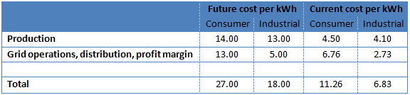Table 8 – expected cost of production for model scenario in the U.S.

The reason behind this lies in the higher cost of all generation technology, but equally in the underutilization of equipment (for example with natural gas generation capacity). Here is the rough calculation we made for the above scenario:

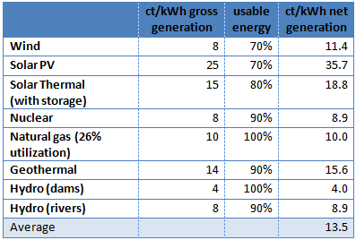Table 9 – expected generation cost in future scenario

What all this shows so far is that even when sticking to the lowest cost option for compensating the intermittency of renewable energy – natural gas – the cost of power becomes likely unbearable for a society as a whole. And with this, we haven’t even solved the problem of depleting natural gas resources, which is something that might well affect the above business model within our lifetimes. After that point, there is – at least until now – no feasible answer for an electricity delivery model that reminds us even faintly of what we are used to nowadays in terms of availability and reliability.

A preliminary conclusion and recommendation

We find it very hard to ignore the fact that all promoted renewable sources currently face and pose significant challenges to the stability of future electricity. So far, many of the planned additions seem almost irrelevant as they add high cost for very little benefit. This problem, however, is currently papered over with increasing use of flexible sources, so it will only really become a problem once we get to the point where fossil fuels, and mainly natural gas, become scarce, or simply too expensive.

For all those who – after all this information – still think that there is a future with smart and super grids, with large shares of renewables and new storage technologies, we are happy to engage in real-life discussions where we go through all the real-life data available. We are talking about a serious problem here and not one of belief.

And, obviously, we are happy to look at new data and new technologies, because we actually hope that something convincing might come our way, but so far to no avail. It is not our objective to “kill” any particular solution or invention, but we are deeply worried about the fact that we are currently using our scarce resources (including money) on things that cannot work.

Based on what we know today, we only see the following possibilities for the future that keep delivery systems halfway intact without creating too much stress for societal systems (and government budgets):

• Stop or reshape large scale investment funding and feed-in support for many renewables and enabling technologies (solar, wave, biomass, smart grids, super grids, and most storage technologies) and instead finance research until proof of concept (including decent EROI and fossil fuel dependence data) has been established for each new technology.
• Focus investment support on the build-out of wind power up to a share of 10-15% of total consumption (or more if ample all-year-round hydropower from reservoirs is available) and match 100% of it (minus the hydropower capacity reliably available all year round) with natural gas generation capacity as backup.
• Couple feed-in tariffs with the ability to deliver steady energy services, encouraging the coupling of either multiple sources by providers and/or supply and demand – before approval for funding. For example, large solar energy producers would be required to match their contribution with AC and water heating equipment that automatically gets turned on and off as supply levels change.
• Send everybody back to the drawing board to think about a) how a future without steady electricity services should and could look like or b) about how we could possibly solve our problem of stocks once fossil fuels run out to maintain stable electricity at a meaningful price.

In our next and final post, we will provide individual technology reviews to show what each generation, storage and demand management technology can provide to future energy systems based on current knowledge.

The entire list of posts in this series can be accessed by clicking on the tag fake fire brigade.